From Real Exams Quiz
Secondary 2 Geography Map Graph Data Skills Quiz
Free Sec 2 Geography Map Graph Data Skills quiz, Nemo3 Exam version, with questions, answers, and syllabus-aligned practice for Singapore students.
These static practice materials are generated from the site's syllabus and paper-generation workflow, with source and model context shown so students and parents can evaluate the material before use.
Questions
Secondary 2 Geography Quiz - Map Graph Data Skills
Name: ________________________
Class: ________________________
Date: ________________________
Score: _____ / 40
Duration: 45 minutes
Total Marks: 40
Instructions:
- Answer all questions in the spaces provided.
- Write your answers clearly and legibly.
- For map-based questions, refer to the map extract provided.
- For graph/data questions, refer to the data provided.
- Marks are indicated in brackets [ ] at the end of each question or part.
Section A: Map Reading Skills (12 marks)
Refer to the map extract of Singapore (Scale 1:50,000) provided for Questions 1–5.
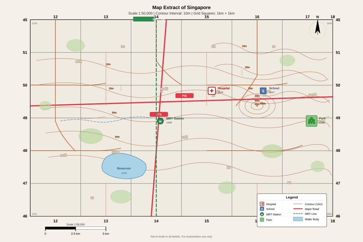
Generated map for Q1.
-
State the four-figure grid reference of the hospital shown on the map. [1]
Answer: ________________________
-
State the six-figure grid reference of the MRT station shown on the map. [1]
Answer: ________________________
-
What is the straight-line distance in kilometres between the school (grid square 1647) and the park (grid square 1750)? [2]
Answer: ________________________ km
-
The contour lines in grid square 1446 are closely spaced, while those in grid square 1750 are widely spaced. What does this difference in contour spacing tell you about the relief (shape of the land) in these two grid squares? [2]
Answer: ________________________
-
A student walks from the hospital (1548) directly to the reservoir (1346). (a) In which general compass direction does the student walk? [1]
Answer: ________________________
(b) If the student walks at an average speed of 5 km/h, estimate how long the journey would take in minutes. Show your working. [2]
Working: ________________________
Answer: ________________________ minutes
Section B: Graph and Data Interpretation (16 marks)
Refer to the climatic graph for Station X provided for Questions 6–10.
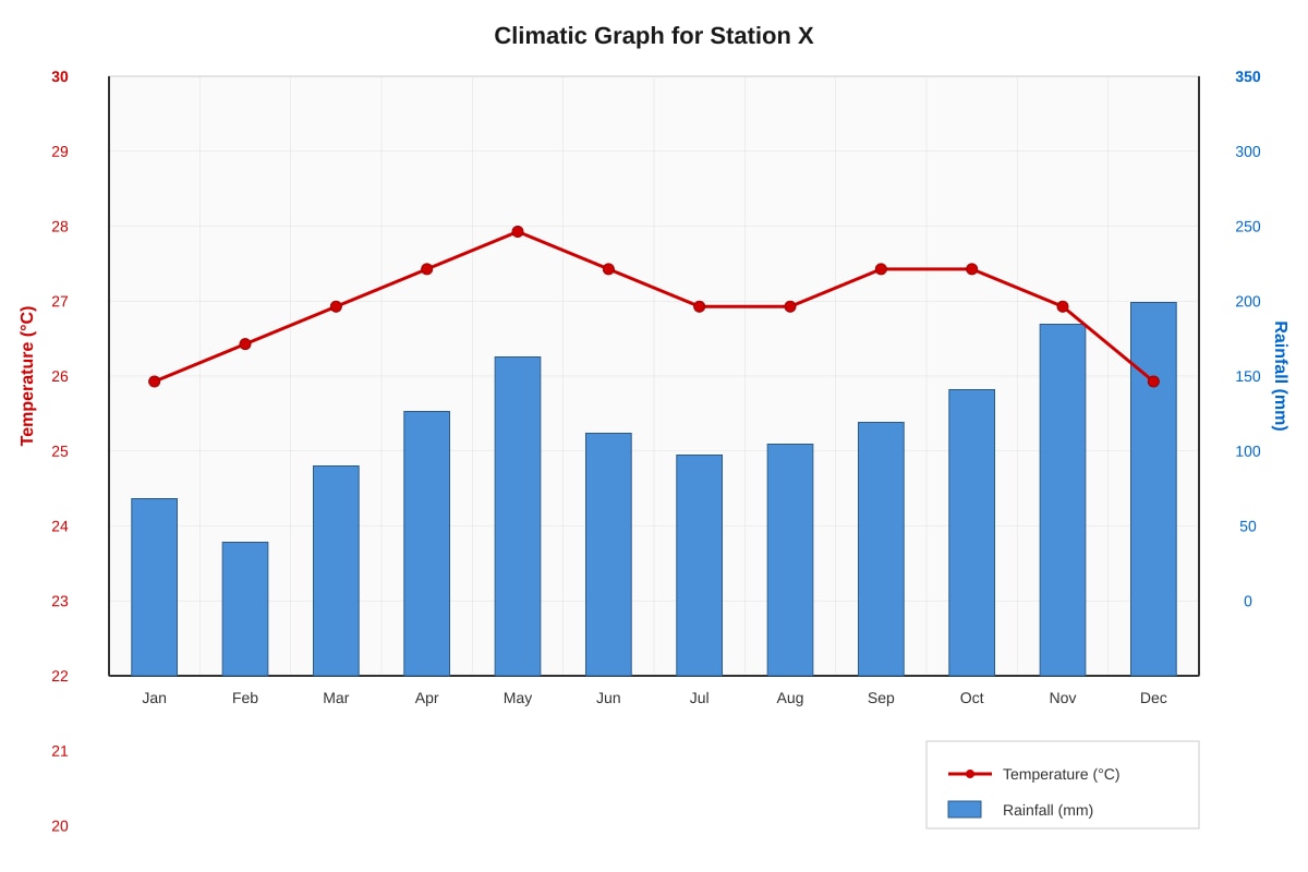
Generated graph for Q6.
-
Which month has the highest temperature? State the temperature. [1]
Answer: ________________________ °C
-
Calculate the annual range of temperature for Station X. [1]
Answer: ________________________ °C
-
Which month receives the highest rainfall? State the rainfall amount. [1]
Answer: ________________________ mm
-
Calculate the total annual rainfall for Station X. Show your working. [2]
Working: ________________________
Answer: ________________________ mm
-
Describe the relationship between temperature and rainfall patterns shown in the graph for Station X. [3]
Answer: ________________________
Refer to the population pyramid for Country Y (2023) provided for Questions 11–13.
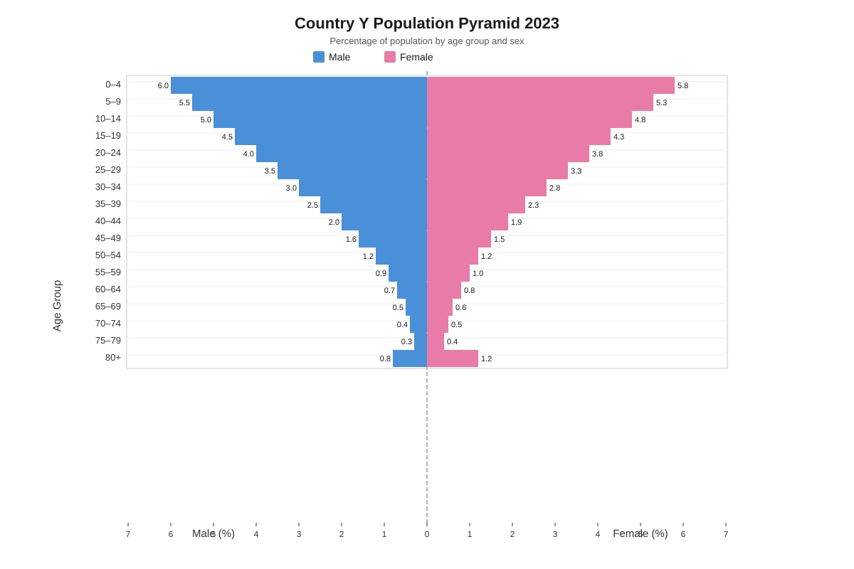
Generated chart for Q11.
-
Describe the shape of the population pyramid for Country Y. What does this shape suggest about the birth rate and death rate of the country? [3]
Answer: ________________________
-
Calculate the percentage of the population aged 0–14 (youth dependency ratio numerator) for Country Y. Show your working. [2]
Working: ________________________
Answer: ________________________ %
-
Country Y is likely a developing or developed country? Use evidence from the population pyramid to support your answer. [2]
Answer: ________________________
Refer to the table below for Questions 14–15.
| Year | Urban Population (%) | Rural Population (%) | Total Population (millions) |
|---|---|---|---|
| 1990 | 35 | 65 | 40 |
| 2000 | 42 | 58 | 52 |
| 2010 | 51 | 49 | 65 |
| 2020 | 58 | 42 | 78 |
-
Calculate the urban population in millions for the year 2010. Show your working. [2]
Working: ________________________
Answer: ________________________ million
-
Describe the trend in urbanisation shown in the table from 1990 to 2020. Suggest one reason for this trend. [3]
Answer: ________________________
Section C: Data Analysis and Application (12 marks)
Refer to the photograph of a coastal landscape provided for Questions 16–18.
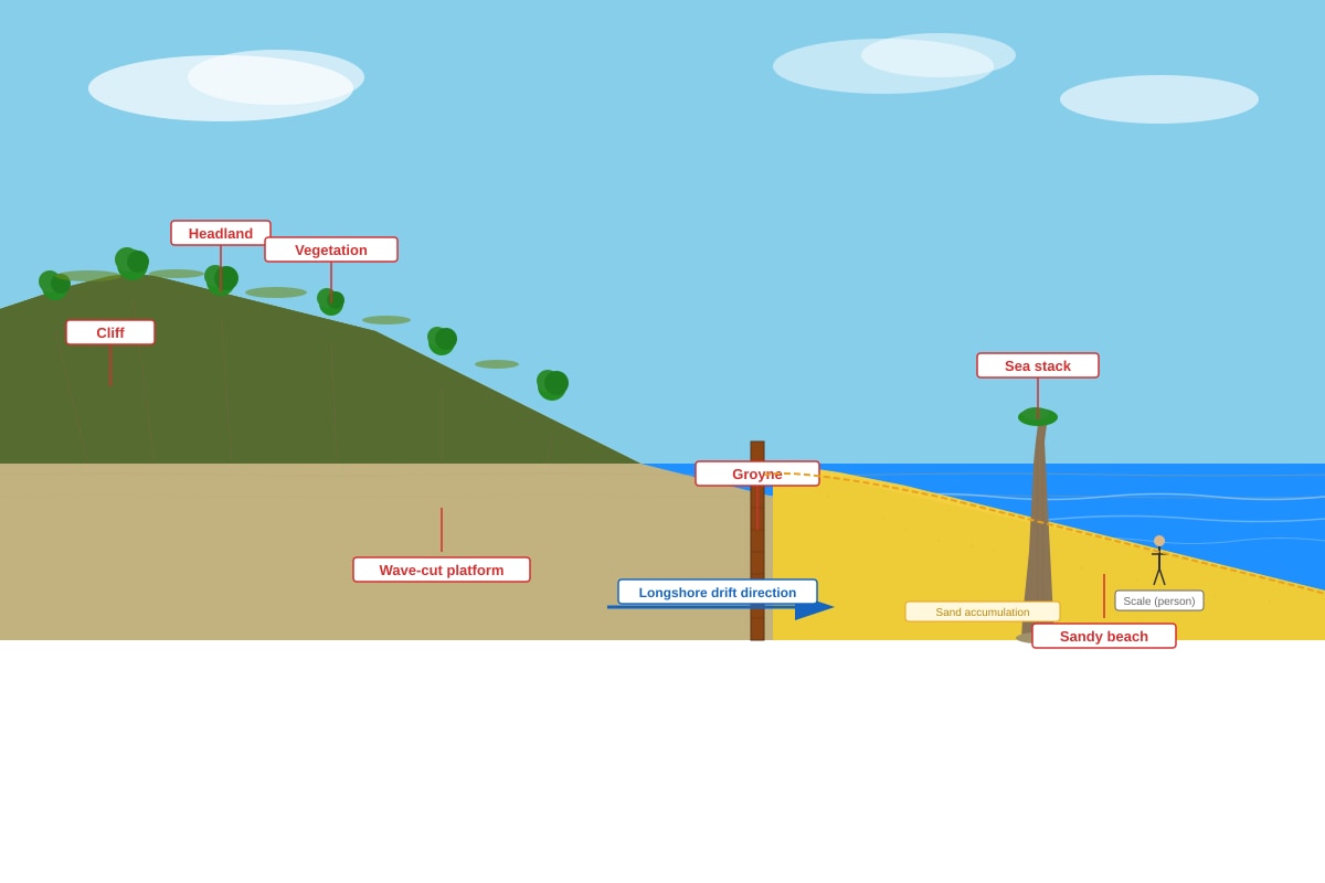
Generated source_image for Q16.
-
Identify the coastal landforms labelled A (cliff), B (wave-cut platform), and C (sea stack) in the photograph. [3]
A: ________________________ B: ________________________ C: ________________________
-
Explain how the sea stack (C) was formed. Use geographical terms in your answer. [3]
Answer: ________________________
-
The photograph shows a groyne on the beach. Explain the purpose of a groyne and how it affects the beach. [2]
Answer: ________________________
Refer to the GIS map screenshot showing land use zones in a city for Questions 19–20.
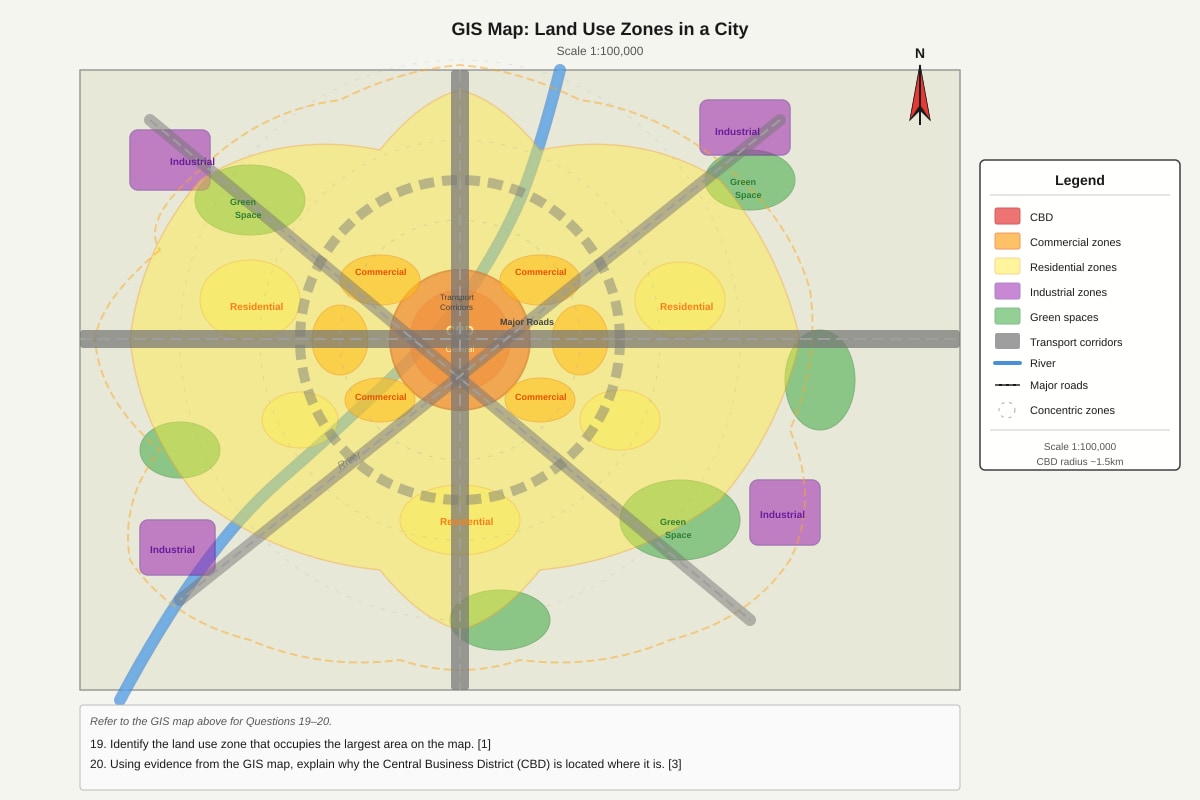
Generated map for Q19.
-
Identify the land use zone that occupies the largest area on the map. [1]
Answer: ________________________
-
Using evidence from the GIS map, explain why the Central Business District (CBD) is located where it is. [3]
Answer: ________________________
End of Quiz
Answers
Secondary 2 Geography Quiz - Map Graph Data Skills (Answer Key)
Total Marks: 40
Section A: Map Reading Skills (12 marks)
Question 1 [1 mark]
Answer: 1548
Explanation: Four-figure grid references are read by stating the easting (vertical grid line) first, then the northing (horizontal grid line). The hospital is located in the grid square where easting 15 meets northing 48.
Common mistake: Writing northing first (4815) or giving a six-figure reference (e.g., 152482).
Question 2 [1 mark]
Answer: 142493 (or 143493 depending on exact position within grid square)
Explanation: Six-figure grid references divide each 1km grid square into 10 tenths (100m each). The MRT station is in grid square 1449. Estimate its position: approximately 2/10 east of easting 14 (→ 142) and 3/10 north of northing 49 (→ 493). Combined: 142493.
Marking note: Accept reasonable estimates (e.g., 141493 to 143493) if the station symbol is centrally placed.
Question 3 [2 marks]
Answer: 3.2 km (accept 3.0–3.5 km)
Working:
- School at 1647 → centre approx. 16.5, 47.5
- Park at 1750 → centre approx. 17.5, 50.5
- Difference in eastings: 1.0 km; difference in northings: 3.0 km
- Straight-line distance = √(1.0² + 3.0²) = √10 ≈ 3.16 km ≈ 3.2 km
Alternative method: Measure with ruler on map (1 cm = 0.5 km at 1:50,000). If distance measures 6.4 cm → 3.2 km.
Mark allocation: 1 mark for correct method/measurement, 1 mark for correct answer with units.
Question 4 [2 marks]
Answer: Closely spaced contours in grid square 1446 indicate steep slopes / high relief (e.g., hillside or valley side). Widely spaced contours in grid square 1750 indicate gentle slopes / low relief (e.g., flat land or plateau).
Mark allocation: 1 mark for interpreting close spacing = steep; 1 mark for interpreting wide spacing = gentle. Must use terms "steep/gentle slope" or "high/low relief".
Question 5 [3 marks total]
(a) [1 mark]
Answer: South-west (SW)
Explanation: Hospital at 1548, reservoir at 1346. Change in easting: 15 → 13 (west). Change in northing: 48 → 46 (south). Combined direction: south-west.
(b) [2 marks]
Working:
- Grid difference: 2 km west, 2 km south → straight-line distance = √(2² + 2²) = √8 ≈ 2.83 km
- Time = Distance ÷ Speed = 2.83 km ÷ 5 km/h = 0.566 hours
- 0.566 × 60 minutes = 33.96 minutes ≈ 34 minutes
Answer: 34 minutes (accept 33–35 minutes)
Mark allocation: 1 mark for correct distance calculation, 1 mark for correct time conversion and answer.
Section B: Graph and Data Interpretation (16 marks)
Question 6 [1 mark]
Answer: May, 28°C
Explanation: Read the temperature line graph. The highest point is in May at 28°C.
Question 7 [1 mark]
Answer: 4°C
Working: Annual range = Highest monthly temperature – Lowest monthly temperature = 28°C (May) – 24°C (Jan/Dec) = 4°C.
Note: Some students mistakenly use Jan (26°C) as lowest; check graph shows 24°C for Jan/Dec.
Question 8 [1 mark]
Answer: December, 300 mm
Explanation: Read the rainfall bar chart. The tallest bar is December at 300 mm.
Question 9 [2 marks]
Working:
Sum of monthly rainfall:
120 + 80 + 150 + 200 + 250 + 180 + 160 + 170 + 190 + 220 + 280 + 300 = 2,300 mm
Answer: 1 mark for correct addition method, 1 mark for correct total.
Answer: 2,300 mm
Question 10 [3 marks]
Answer: Station X shows consistently high temperatures throughout the year (range only 4°C, 26–28°C), typical of equatorial regions. Rainfall is high every month (minimum 80 mm in February), with no distinct dry month. Rainfall peaks in November–December (280–300 mm) and has a secondary peak in April–May (200–250 mm), suggesting a double rainfall maximum possibly linked to monsoon transitions. Temperature peaks slightly before the main rainfall peaks (May 28°C before Nov–Dec rainfall peak).
Mark allocation:
- 1 mark: Describe temperature pattern (uniform, high, small range)
- 1 mark: Describe rainfall pattern (high year-round, no dry month, peaks)
- 1 mark: Identify relationship (temp peaks before rainfall peaks / double rainfall maxima)
Key concept: Equatorial climate characteristics.
Question 11 [3 marks]
Answer: The population pyramid has a broad base (0–4 age group: ~11.8% combined) and narrows steadily towards the top (80+: ~2.0% combined), forming a classic expansive/pyramid shape. This indicates a high birth rate (wide base = many young children) and a high death rate (rapid narrowing = fewer people survive to old age), typical of a country in Stage 2 of the Demographic Transition Model. Life expectancy is relatively low.
Mark allocation:
- 1 mark: Describe shape (broad base, narrow top, pyramid/expansive)
- 1 mark: Link to high birth rate
- 1 mark: Link to high death rate / low life expectancy
Question 12 [2 marks]
Working:
Sum of percentages for age groups 0–4, 5–9, 10–14 (both sexes):
Males: 6.0 + 5.5 + 5.0 = 16.5%
Females: 5.8 + 5.3 + 4.8 = 15.9%
Total youth (0–14) = 16.5% + 15.9% = 32.4%
Answer: 32.4%
Mark allocation: 1 mark for correct identification of age groups and addition method, 1 mark for correct total.
Question 13 [2 marks]
Answer: Country Y is likely a developing country. Evidence: (1) Broad base of pyramid shows high birth rate, common in developing countries with limited access to family planning/education for women. (2) Rapid narrowing indicates high infant/child mortality and lower life expectancy due to limited healthcare. (3) Small elderly population (80+ only ~2%) reflects lower life expectancy.
Mark allocation: 1 mark for correct classification (developing), 1 mark for valid evidence from pyramid (birth rate, death rate, or life expectancy).
Question 14 [2 marks]
Working:
Urban population 2010 = 51% of 65 million = 0.51 × 65 = 33.15 million
Answer: 33.15 million (accept 33.2 million or 33 million)
Mark allocation: 1 mark for correct formula (percentage × total), 1 mark for correct calculation and units.
Question 15 [3 marks]
Answer: Trend: Urban population percentage increased steadily from 35% (1990) to 58% (2020), while rural percentage decreased from 65% to 42%. In absolute numbers, urban population grew from 14 million (0.35×40) to 45.24 million (0.58×78) – more than a threefold increase.
Reason: Rural-to-urban migration driven by pull factors such as better employment opportunities in manufacturing/services, better access to education/healthcare, and higher wages in cities. Push factors include mechanisation of agriculture reducing rural jobs, and land scarcity.
Mark allocation: 1 mark for describing trend (with data), 1 mark for describing magnitude of change, 1 mark for valid reason (push/pull factor).
Section C: Data Analysis and Application (12 marks)
Question 16 [3 marks]
Answer:
A: Cliff (steep rock face at coastline)
B: Wave-cut platform (flat rocky surface at base of cliff, exposed at low tide)
C: Sea stack (isolated pillar of rock standing offshore, detached from headland)
Mark allocation: 1 mark per correct identification. Accept "wave-cut notch" for B if at cliff base, but "wave-cut platform" is the visible flat surface.
Question 17 [3 marks]
Answer: The sea stack forms through coastal erosion on a headland:
- Hydraulic action and abrasion widen cracks in the headland, forming a cave.
- The cave erodes through the headland to form an arch.
- Continued erosion enlarges the arch until the roof collapses due to gravity and lack of support.
- The remaining isolated pillar of rock is the sea stack. Over time, the stack will further erode to a stump.
Mark allocation: 1 mark for sequence (cave → arch → stack), 1 mark for naming processes (hydraulic action, abrasion, gravity/collapse), 1 mark for mentioning headland context and eventual stump formation.
Question 18 [2 marks]
Answer: A groyne is a low wall built perpendicular to the shore to trap sediment moved by longshore drift. It interrupts the alongshore movement of sand, causing accumulation (build-up) on the updrift side (where waves approach from) and erosion on the downdrift side. This widens the beach locally, protecting the cliff or land behind from wave attack.
Mark allocation: 1 mark for purpose (trap longshore drift sediment / widen beach), 1 mark for effect (build-up on one side, erosion on other / protects coast).
Question 19 [1 mark]
Answer: Residential (yellow zone)
Explanation: On the GIS map, the yellow residential zone extends from the CBD outward to ~8 km radius, covering the largest surface area compared to the compact CBD, industrial corridors, and scattered green spaces.
Question 20 [3 marks]
Answer: The CBD is located at the centre of the transport network (major roads and rail lines converge here), making it the most accessible location for workers, shoppers, and businesses. It sits at the intersection of transport corridors and alongside the river (historical transport route). Land values are highest here due to accessibility, so only high-revenue activities (offices, retail, finance) can afford the rent, creating the characteristic high-density, vertical land use. The concentric residential zones around it confirm the CBD as the focal point of the urban model (Burgess concentric zone model).
Mark allocation: 1 mark for accessibility/transport convergence, 1 mark for high land value/bid-rent concept, 1 mark for reference to urban model or map evidence (river, transport, centrality).
End of Answer Key
Free quiz and exam paper access
Enter your details to view this paper
Your access is remembered on this device.