AI Generated Exam Paper
Secondary 1 Geography Practice Paper 2
Free Sec 1 Geography Practice Paper 2, Nemo3 AI version, with questions, answers, and syllabus-aligned practice for Singapore students.
These static practice materials are generated from the site's syllabus and paper-generation workflow, with source and model context shown so students and parents can evaluate the material before use.
Questions
TuitionGoWhere Practice Paper - Geography Secondary 1
TuitionGoWhere Practice Paper (AI) — Version 2
Subject: Geography
Level: Secondary 1
Paper: Practice Paper 2 (Map, Graph & Data Skills)
Duration: 1 hour 15 minutes
Total Marks: 50
Name: ___________________________
Class: ___________________________
Date: ___________________________
Instructions to Candidates
- Answer all questions.
- Write your answers in the spaces provided.
- The number of marks is given in brackets [ ] at the end of each question or part question.
- The total number of marks for this paper is 50.
- You may use a calculator.
- For map-based questions, refer to the map extract provided in the image placeholders.
Section A: Map Skills [20 marks]
Question 1
Study the map extract of Tampines Town provided below. The map uses a scale of 1 : 25 000.
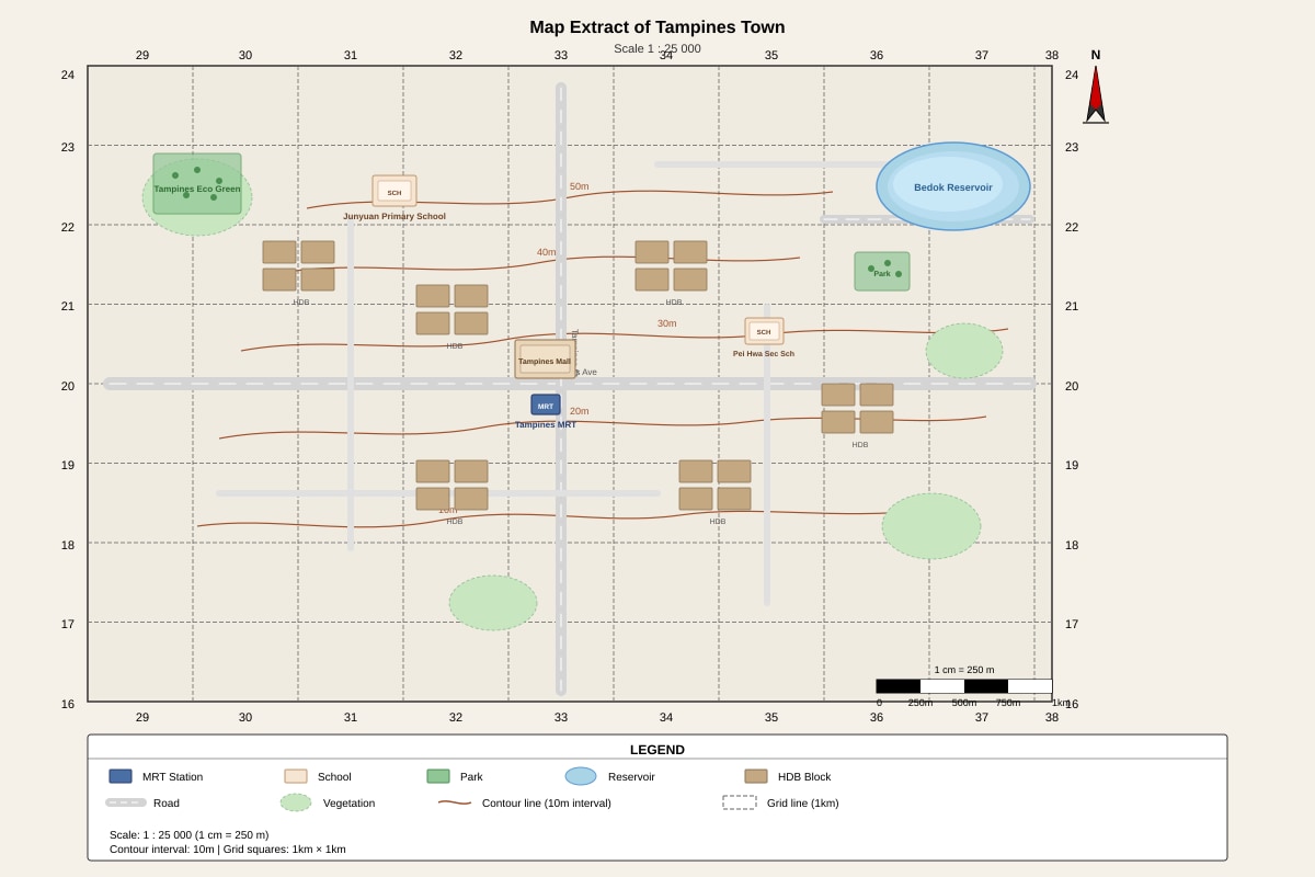
Generated map for Q1.
(a) State the four-figure grid reference of Tampines MRT Station.
[1]
(b) State the six-figure grid reference of Junyuan Primary School.
[1]
(c) What is the direction of Bedok Reservoir from Tampines Mall?
[1]
Question 2
The map extract shows contour lines at 10-metre intervals.
(a) What is the height of the highest point shown in grid square 3121?
[1]
(b) Describe the relief (shape of the land) in grid square 3020. Use evidence from the contour lines to support your answer.
[2]
(c) Calculate the average gradient of the slope between the 20 m contour line and the 30 m contour line along a straight line running east-west across grid square 3121, if the horizontal distance between these two contour lines on the map is 0.8 cm.
Show your working clearly.
[3]
Question 3
Measure the straight-line distance between Tampines MRT Station and the centre of Bedok Reservoir on the map.
Give your answer in kilometres.
Show your working.
[2]
Question 4
A new cycling path is proposed to run from Tampines Eco Green (grid square 3122) to Bedok Reservoir Park (grid square 3120).
(a) Using evidence from the map, suggest one advantage and one disadvantage of routing the cycling path along the existing park connector network (shown as dashed green lines) compared to a straight-line route across the reservoir.
[2]
(b) The straight-line distance across the reservoir is 1.2 km. If a cyclist travels at an average speed of 15 km/h, how long in minutes would it take to cross the reservoir?
[1]
Question 5
The map shows several land-use zones in Tampines Town.
(a) Identify the dominant land use in grid square 3021.
[1]
(b) Explain one reason why this land use is located near the MRT station.
[2]
Section B: Graph & Data Interpretation [18 marks]
Question 6
The table below shows the monthly rainfall (in mm) recorded at a weather station in Singapore for the first six months of 2023.
| Month | Jan | Feb | Mar | Apr | May | Jun |
|---|---|---|---|---|---|---|
| Rainfall (mm) | 210 | 110 | 185 | 245 | 195 | 160 |
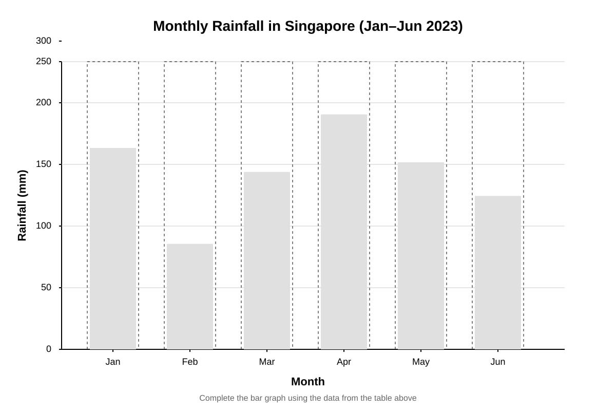
Generated graph for Q6.
(a) Using the data in the table, complete the bar graph on the axes provided above.
[2]
(b) Which month had the highest rainfall?
[1]
(c) Calculate the mean monthly rainfall for these six months.
Show your working.
[2]
(d) The annual rainfall for 2023 was 2,650 mm. What percentage of the annual rainfall fell in the first six months?
Give your answer to one decimal place.
[2]
Question 7
The divided bar graph below shows the percentage composition of water sources for Singapore's water supply in two different years.
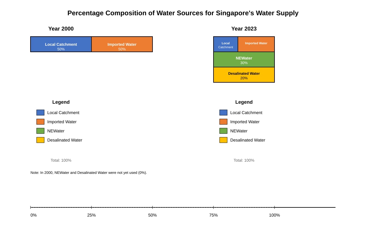
Generated chart for Q7.
(a) State the percentage of NEWater in Singapore's water supply in 2023.
[1]
(b) Calculate the increase in percentage of desalinated water from 2000 to 2023.
[1]
(c) Describe the trend in the use of imported water between 2000 and 2023.
[1]
(d) Explain one geographical reason why Singapore has increased its use of NEWater and desalinated water.
[2]
(e) If Singapore's total daily water demand in 2023 was 1,900 million litres, calculate the volume of water supplied by NEWater per day in million litres.
[1]
Question 8
A student conducted a traffic count at a junction near a secondary school for 30 minutes during the morning peak (7:00–7:30 am). The results are shown below.
| Vehicle Type | Number Counted |
|---|---|
| Cars | 120 |
| Buses | 15 |
| Motorcycles | 45 |
| Bicycles | 30 |
| Lorries/Vans | 20 |
| Total | 230 |
(a) Calculate the percentage of cars out of the total vehicles counted.
Give your answer to one decimal place.
[1]
(b) The student wants to present this data using a pie chart. Calculate the angle of the sector for motorcycles.
Show your working.
[2]
(c) Suggest one limitation of using this 30-minute count to understand the daily traffic pattern at this junction.
[1]
Section C: Data Analysis & Geographical Skills [12 marks]
Question 9
The table below shows population density and green space per person for four towns in Singapore.
| Town | Population Density (persons/km²) | Green Space per Person (m²) |
|---|---|---|
| A | 12,500 | 8.2 |
| B | 8,200 | 14.5 |
| C | 15,800 | 5.1 |
| D | 10,400 | 11.3 |
(a) Which town has the highest population density?
[1]
(b) Plot a scatter graph on the axes below to show the relationship between population density and green space per person.
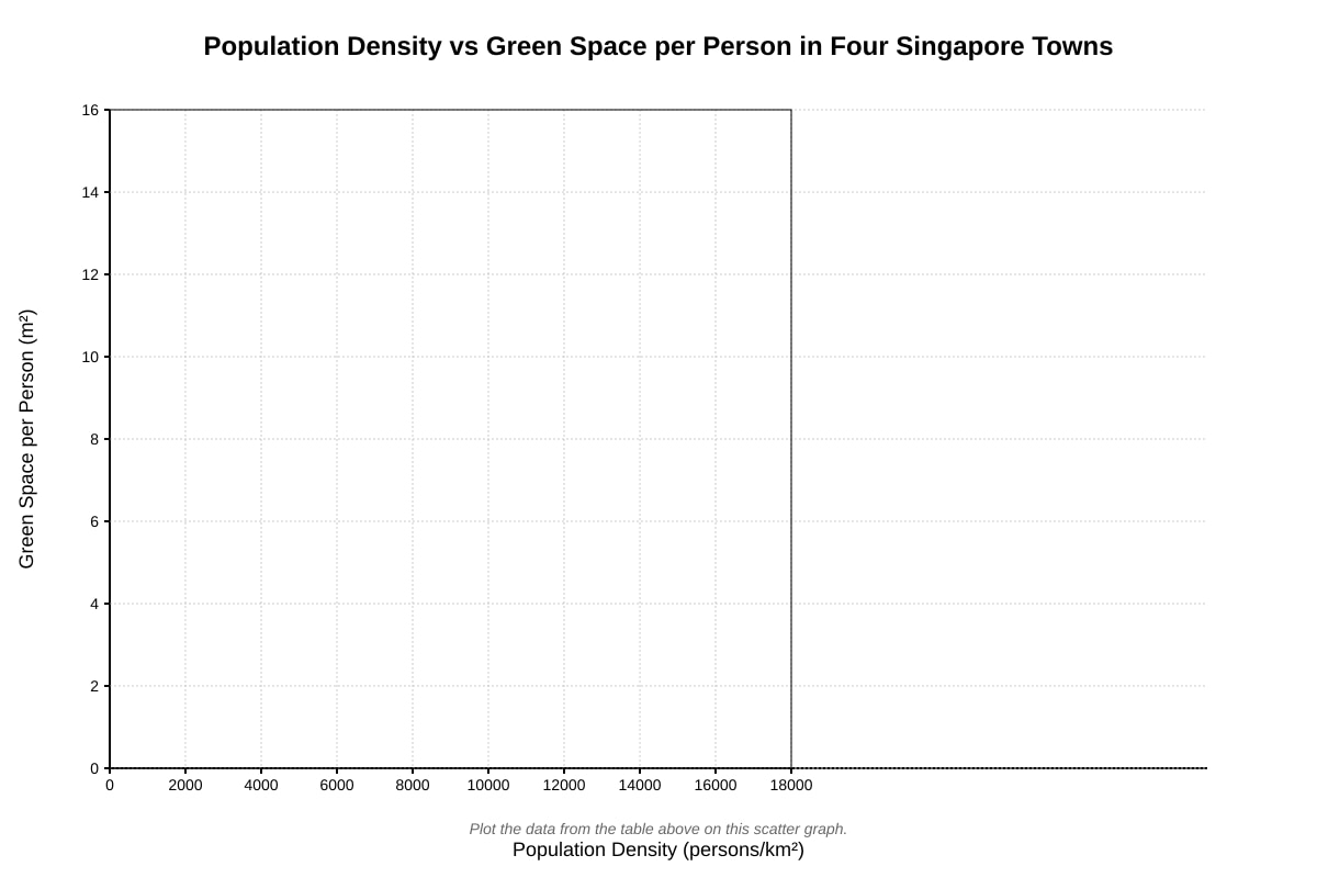
Generated graph for Q9.
[2]
(c) Describe the relationship shown by the scatter graph.
[1]
(d) Town E has a population density of 13,000 persons/km². Based on the trend, estimate the green space per person for Town E.
[1]
(e) Explain one reason why towns with higher population density tend to have less green space per person.
[2]
Question 10
The climate graph below shows the monthly temperature and rainfall for a location in Singapore.
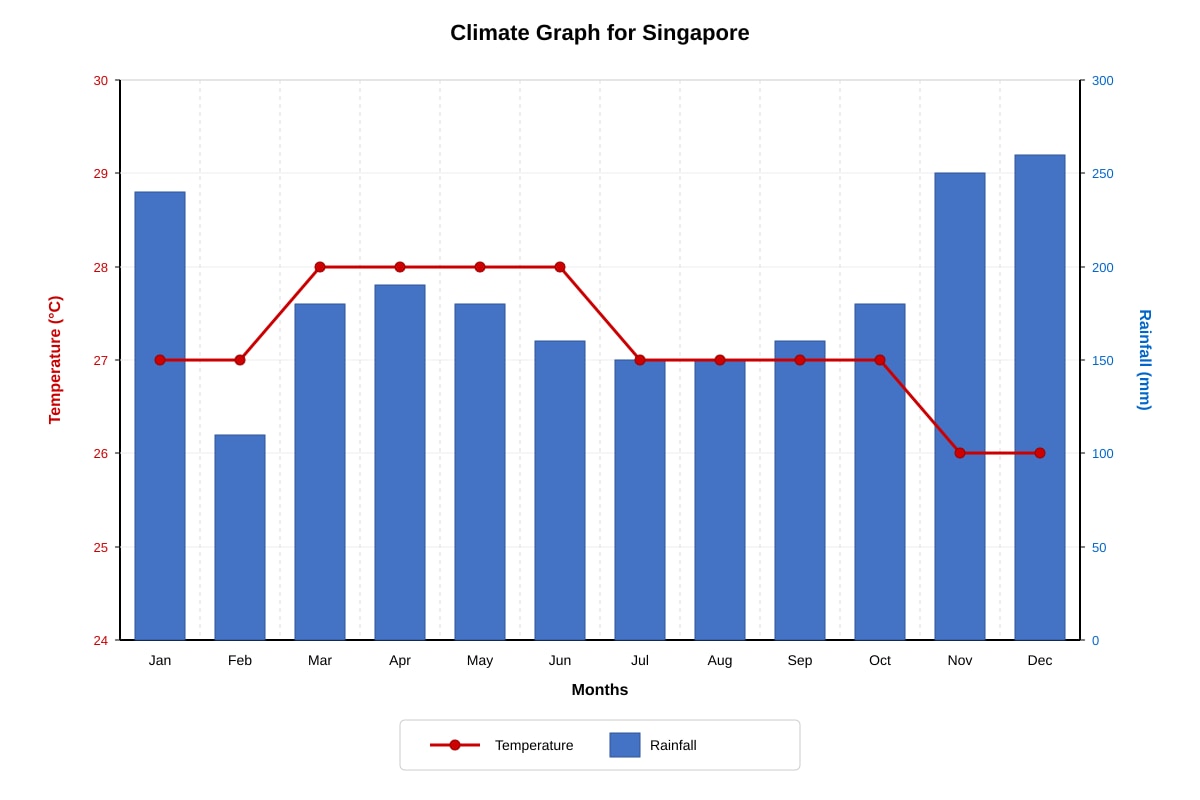
Generated graph for Q10.
(a) State the month with the highest rainfall.
[1]
(b) Calculate the annual temperature range for this location.
[1]
(c) Describe the rainfall pattern throughout the year.
[2]
(d) Explain why Singapore experiences this type of rainfall pattern.
[2]
Question 11
A Geography student is investigating water quality at two sites along a river: Site X (upstream) and Site Y (downstream). The results are shown below.
| Parameter | Site X (Upstream) | Site Y (Downstream) |
|---|---|---|
| Dissolved Oxygen (mg/L) | 8.5 | 4.2 |
| Biochemical Oxygen Demand (mg/L) | 1.2 | 6.8 |
| Nitrate Concentration (mg/L) | 0.5 | 12.3 |
| pH | 7.2 | 6.5 |
| Turbidity (NTU) | 5 | 45 |
(a) Which site has better water quality? Support your answer with two pieces of evidence from the table.
[2]
(b) Suggest one human activity at or near Site Y that could explain the differences in water quality.
[1]
(c) Explain why Biochemical Oxygen Demand (BOD) is higher at Site Y.
[2]
End of Paper
Answers
TuitionGoWhere Practice Paper - Geography Secondary 1 (Answer Key)
TuitionGoWhere Practice Paper (AI) — Version 2
Subject: Geography
Level: Secondary 1
Paper: Practice Paper 2 (Map, Graph & Data Skills)
Total Marks: 50
Section A: Map Skills [20 marks]
Question 1
(a) 3121
Method: Read eastings first (vertical grid lines): 31. Then read northings (horizontal grid lines): 21. The MRT station symbol lies in the grid square bounded by eastings 31–32 and northings 21–22. The four-figure grid reference is the lower-left corner: 3121.
[1]
(b) 315215
Method: For six-figure grid reference, divide the grid square into 10 tenths. Junyuan Primary School is approximately 5 tenths east of easting 31 → 315. It is approximately 5 tenths north of northing 21 → 215. Combined: 315215.
[1]
(b) North-west (or NW)
Method: Locate Tampines Mall (approx. 3121) and Bedok Reservoir (approx. 3120). The reservoir lies to the north and slightly west of the mall. Accept north, north-west, or northwest.
[1]
Question 2
(a) 30 m
Method: The highest contour line shown in grid square 3121 is labelled 30 m. Contour interval is 10 m.
[1]
(b) Gentle slope / low-lying flat land — Contour lines are widely spaced (or absent / very far apart), indicating gentle gradient or flat terrain.
Evidence: In grid square 3020, contour lines are far apart / only the 10 m contour is visible, showing land is low and flat.
[2]
Mark breakdown: 1 mark for correct relief description (gentle slope/flat), 1 mark for evidence from contour spacing.
(c) Gradient = 1 : 41.7 (or 1 : 42)
Working:
- Vertical interval (VI) = 30 m – 20 m = 10 m
- Horizontal distance on map = 0.8 cm
- Scale = 1 : 25 000 → 1 cm on map = 25 000 cm = 250 m on ground
- Horizontal distance on ground (HE) = 0.8 × 250 m = 200 m
- Gradient = VI : HE = 10 m : 200 m = 1 : 20
Wait — correction: Gradient is expressed as 1 : (HE/VI) = 1 : (200/10) = 1 : 20
But standard format: 1 : 20 (or 1/20)
Recheck: Gradient = Vertical Rise / Horizontal Run = 10 / 200 = 1/20 → 1 : 20
[3]
Mark breakdown: 1 mark for correct VI (10 m), 1 mark for correct HE conversion (200 m), 1 mark for correct gradient ratio (1:20).
Common error: Forgetting to convert map distance to ground distance using scale.
Question 3
Distance = 1.75 km (accept 1.7 – 1.8 km)
Working:
- Measure straight-line distance on map between Tampines MRT (3121) and centre of Bedok Reservoir (3120) → approx. 7.0 cm (accept 6.8–7.2 cm)
- Scale: 1 cm = 250 m (since 1:25 000)
- Ground distance = 7.0 cm × 250 m/cm = 1,750 m = 1.75 km
[2]
Mark breakdown: 1 mark for correct map measurement (with units), 1 mark for correct conversion to km.
Question 4
(a)
Advantage: Safer and more pleasant — Park connectors are separated from vehicular traffic, passing through green spaces (Tampines Eco Green), providing a scenic and safe route for cyclists.
Disadvantage: Longer distance — The park connector network follows a winding path along parks and roads, making the route longer than a straight line across the reservoir.
[2]
Mark breakdown: 1 mark for valid advantage with map evidence, 1 mark for valid disadvantage with map evidence.
(b) 4.8 minutes
Working:
- Distance = 1.2 km
- Speed = 15 km/h
- Time = Distance / Speed = 1.2 / 15 = 0.08 hours
- Convert to minutes: 0.08 × 60 = 4.8 minutes
[1]
Question 5
(a) Residential / High-density housing (HDB flats)
Evidence: Grid square 3021 shows dense building symbols and labels for HDB blocks.
[1]
(b) Accessibility / Transport connectivity — Being near the MRT station allows residents easy access to public transport for commuting to work/school, reducing reliance on private vehicles and supporting sustainable urban living.
Alternative: Convenience — Proximity to MRT and commercial amenities (Tampines Mall) makes the location highly desirable for housing.
[2]
Mark breakdown: 1 mark for identifying reason (accessibility/convenience), 1 mark for explanation linked to urban planning/sustainability.
Section B: Graph & Data Interpretation [18 marks]
Question 6
(a) Graph completion: Six bars drawn to correct heights:
Jan: 210, Feb: 110, Mar: 185, Apr: 245, May: 195, Jun: 160 (mm)
[2]
Mark breakdown: 1 mark for all 6 bars plotted at correct heights (±5 mm tolerance), 1 mark for bars drawn neatly with consistent width and labelled.
(b) April (245 mm)
[1]
(c) Mean = 184.2 mm
Working:
Sum = 210 + 110 + 185 + 245 + 195 + 160 = 1,105 mm
Mean = 1,105 ÷ 6 = 184.166... ≈ 184.2 mm (1 decimal place)
[2]
Mark breakdown: 1 mark for correct sum (1105), 1 mark for correct division and answer to 1 d.p.
(d) 41.7%
Working:
Total Jan–Jun rainfall = 1,105 mm
Annual rainfall = 2,650 mm
Percentage = (1,105 ÷ 2,650) × 100 = 41.698...% ≈ 41.7% (1 d.p.)
[2]
Mark breakdown: 1 mark for correct fraction setup, 1 mark for correct percentage to 1 d.p.
Question 7
(a) 30%
[1]
(b) 20 percentage points (from 0% to 20%)
[1]
(c) Decreased from 50% (2000) to 30% (2023) — a decrease of 20 percentage points.
[1]
(d) To enhance water security and self-sufficiency — Singapore has limited land for catchment and relies on imported water (from Malaysia) which is subject to treaty agreements and geopolitical uncertainty. Developing NEWater (recycled water) and desalination provides weather-resilient, locally controlled sources, reducing vulnerability to supply disruptions.
[2]
Mark breakdown: 1 mark for identifying water security/self-sufficiency, 1 mark for explaining why NEWater/desalination achieve this (local, weather-independent).
(e) 570 million litres
Working:
30% of 1,900 million litres = 0.30 × 1,900 = 570 million litres
[1]
Question 8
(a) 52.2%
Working:
(120 ÷ 230) × 100 = 52.1739...% ≈ 52.2% (1 d.p.)
[1]
(b) 70.4° (accept 70° or 70.4°)
Working:
Motorcycles = 45 out of 230 total
Angle = (45 ÷ 230) × 360° = 70.434...° ≈ 70.4°
[2]
Mark breakdown: 1 mark for correct fraction (45/230), 1 mark for correct multiplication by 360° and answer.
(c) The 30-minute count only captures morning peak traffic and does not reflect traffic patterns at other times (e.g., midday, evening, night), so it cannot represent the daily variation in volume or vehicle composition.
Alternative: Not representative — Single short-duration count may be affected by unusual events (accident, weather, school event).
[1]
Section C: Data Analysis & Geographical Skills [12 marks]
Question 9
(a) Town C (15,800 persons/km²)
[1]
(b) Scatter graph: Four points plotted correctly:
A (12500, 8.2), B (8200, 14.5), C (15800, 5.1), D (10400, 11.3)
[2]
Mark breakdown: 1 mark for all 4 points plotted accurately (±½ grid square), 1 mark for points clearly marked (e.g., with × or dots) and labelled A/B/C/D.
(c) Negative correlation — As population density increases, green space per person decreases.
[1]
(d) Approximately 7.5 m² (accept 7 – 8 m²)
Method: Town E (13,000) lies between Town A (12,500, 8.2) and Town C (15,800, 5.1). By visual interpolation on the trend, green space ≈ 7.5 m².
[1]
(e) Competition for limited land — In high-density towns, land is scarce and expensive. Priority is given to housing, transport, and commercial uses to accommodate more people. Green space is often reduced or fragmented because it does not generate direct economic return and requires large contiguous areas, which are unavailable in built-up zones.
[2]
Mark breakdown: 1 mark for land scarcity/competition, 1 mark for explaining why green space loses out (economic priority, space needs).
Question 10
(a) December (260 mm) — accept November (250 mm) if graph reading varies slightly, but December is highest at 260 mm
[1]
(b) 2 °C
Working: Highest monthly temp = 28°C (Mar–Jun), Lowest = 26°C (Nov–Dec)
Range = 28 – 26 = 2 °C
[1]
(c) High rainfall throughout the year with two peaks: a major peak in November–December (Northeast Monsoon) and a secondary peak in April–May (inter-monsoon). Relatively drier in February and June–August (Southwest Monsoon), but no truly dry month (all months > 100 mm).
[2]
Mark breakdown: 1 mark for identifying two peaks / year-round rain, 1 mark for naming drier months or monsoon seasons.
(d) Equatorial location — Singapore lies near the equator (1°N), experiencing high temperatures year-round which drives intense convection. Rising warm, moist air cools and condenses, causing frequent convectional rainfall. The Intertropical Convergence Zone (ITCZ) shifts across Singapore twice a year (around April and October), bringing heavy rain during monsoon transitions.
[2]
Mark breakdown: 1 mark for equatorial location/convection, 1 mark for ITCZ/monsoon explanation.
Question 11
(a) Site X (Upstream) has better water quality.
Evidence 1: Higher Dissolved Oxygen (8.5 mg/L vs 4.2 mg/L) — indicates healthier aquatic ecosystem.
Evidence 2: Lower BOD (1.2 mg/L vs 6.8 mg/L) — indicates less organic pollution.
Other valid evidence: Lower nitrate (0.5 vs 12.3 mg/L), lower turbidity (5 vs 45 NTU), pH closer to neutral (7.2 vs 6.5).
[2]
Mark breakdown: 1 mark for correct site, 1 mark for two correct pieces of evidence with data.
(b) Discharge of untreated / partially treated sewage or industrial effluent or agricultural runoff (fertilizers) from nearby urban/industrial/farm areas.
Most likely for Singapore context: Urban runoff / sewage discharge from residential/industrial areas downstream.
[1]
(c) Higher BOD at Site Y indicates more organic matter in the water. This is likely due to sewage or organic waste discharge downstream. Bacteria decompose this organic matter, consuming dissolved oxygen in the process, which raises BOD and lowers DO (as seen in the data: DO drops from 8.5 to 4.2 mg/L).
[2]
Mark breakdown: 1 mark for linking BOD to organic matter decomposition, 1 mark for explaining the oxygen consumption process and link to lower DO.
End of Answer Key
Free quiz and exam paper access
Enter your details to view this paper
Your access is remembered on this device.