AI Generated Exam Paper
Secondary 1 Geography Practice Paper 2
Free Sec 1 Geography Practice Paper 2, Kimi2.6 AI version, with questions, answers, and syllabus-aligned practice for Singapore students.
These static practice materials are generated from the site's syllabus and paper-generation workflow, with source and model context shown so students and parents can evaluate the material before use.
Questions
TuitionGoWhere Practice Paper - Geography Secondary 1
TuitionGoWhere Practice Paper (AI)
Version: 2 of 5
| Subject: | Geography |
| Level: | Secondary 1 |
| Paper: | Practice Paper (Map Skills, Data Interpretation & Geographical Inquiry) |
| Duration: | 1 hour 15 minutes |
| Total Marks: | 60 |
| Name: | _________________________________ |
| Class: | _________________________________ |
| Date: | _________________________________ |
Instructions to Candidates
- Write your name, class, and date in the spaces provided above.
- Answer all questions.
- Write your answers in the spaces provided. If you need extra space, use the blank pages at the end of this paper.
- For questions requiring calculations, show all your working clearly.
- Read each question carefully and note the command words used (e.g., state, describe, explain, compare).
- The use of calculators is not permitted for this paper.
- The number of marks is shown in brackets [ ] at the end of each question or part question.
Section A: Map Skills and Spatial Data
Total: 20 marks | Suggested time: 25 minutes
Generated map for Q1-Q5.
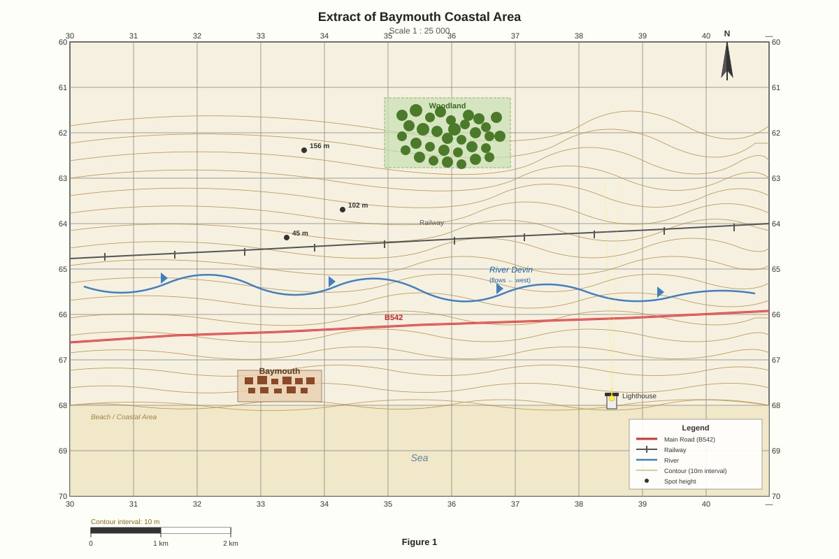
1. Study Figure 1, the map extract of Baymouth Coastal Area.
(a) State the 4-figure grid reference of the settlement of Baymouth.
_______________________________________________ [1]
(b) State the 6-figure grid reference of the spot height 156 m.
_______________________________________________ [1]
(c) In which compass direction does the River Devin flow? Explain how you determined this.
_______________________________________________
_______________________________________________
_______________________________________________ [2]
(d) Calculate the straight-line distance, in kilometres, between the spot height 45 m and the spot height 102 m. Show your working.
_______________________________________________
_______________________________________________
_______________________________________________ [3]
(e) Describe the relief (shape of the land) in grid square 3466.
_______________________________________________
_______________________________________________ [2]
2. Study Figure 1.
(a) Identify the type of road shown by the symbol at grid reference 3364.
_______________________________________________ [1]
(b) Name the human feature found at 6-figure grid reference 338663.
_______________________________________________ [1]
(c) Suggest one reason why the railway line was built along its current route rather than taking a more direct path across the higher land.
_______________________________________________
_______________________________________________ [2]
3.
Generated map for Q3.
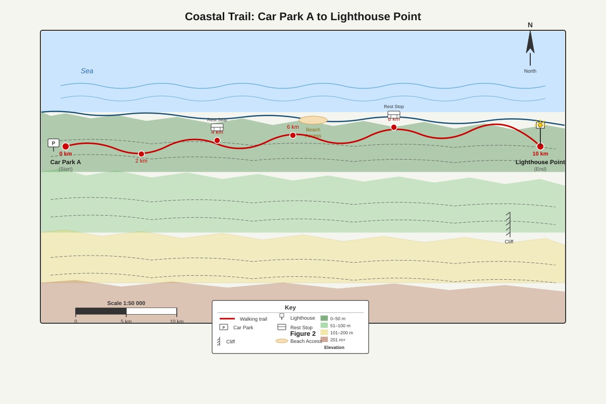
Study Figure 2, the tourist route map of a coastal walking trail.
(a) What is the total length of the walking trail from Car Park A to Lighthouse Point?
_______________________________________________ [1]
(b) Calculate the horizontal equivalent distance on the ground, in metres, represented by 2 cm on this map. Show your working.
_______________________________________________
_______________________________________________ [2]
(c) A walker completes the trail in 3 hours. Calculate the average walking speed in km/h.
_______________________________________________
_______________________________________________ [2]
4. Study Figure 2.
(a) Describe the elevation pattern along the trail from start to finish.
_______________________________________________
_______________________________________________
_______________________________________________ [2]
(b) Explain why the final 2 km of the trail might be the most challenging section for walkers.
_______________________________________________
_______________________________________________ [2]
Section A Total: 20 marks
Section B: Graph and Data Interpretation
Total: 24 marks | Suggested time: 30 minutes
5.
Generated graph for Q5.
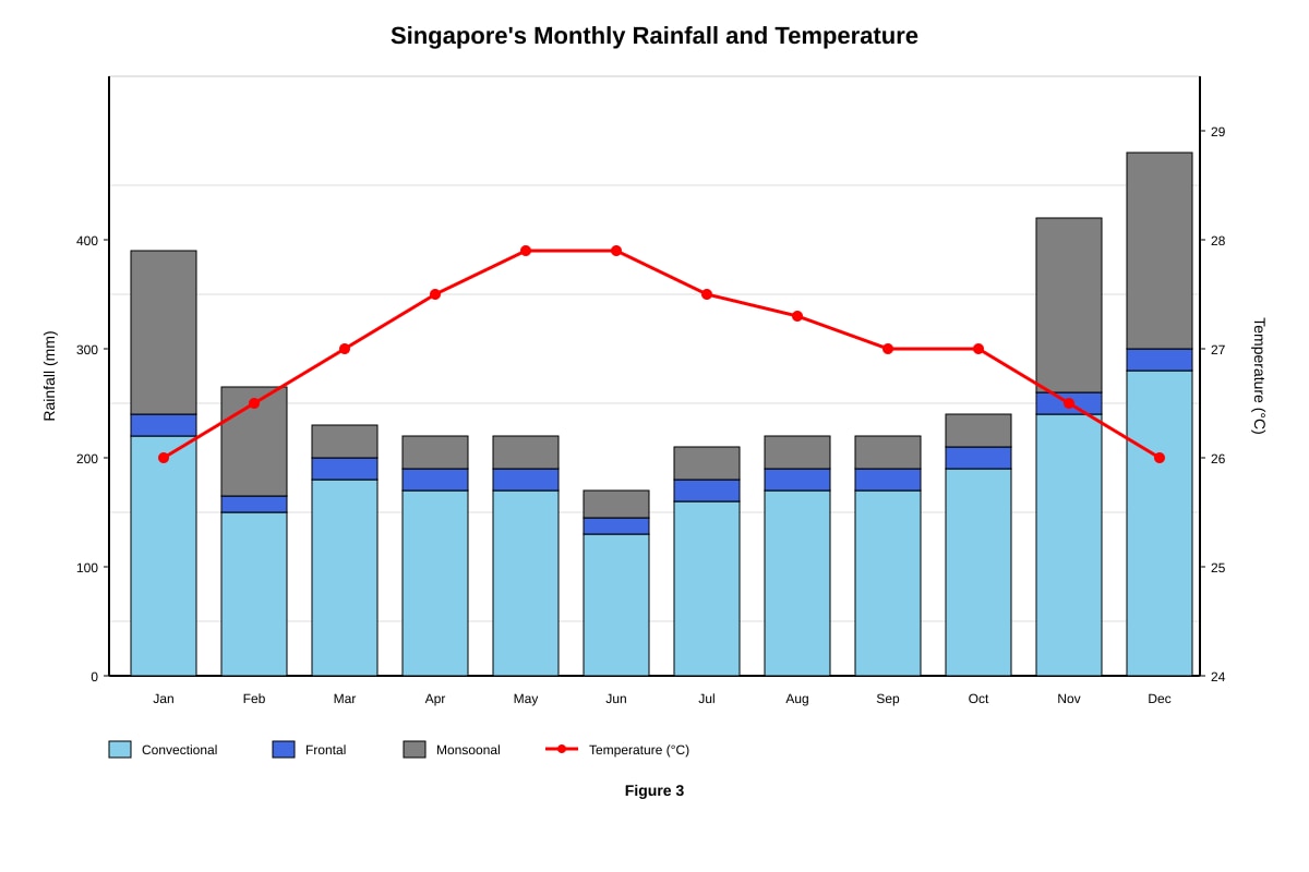
Study Figure 3, which shows Singapore's monthly rainfall and temperature.
(a) State the total rainfall, in mm, for the month of November.
_______________________________________________ [1]
(b) Identify the wettest three-month period and the driest three-month period.
Wettest: _______________________________________
Driest: ________________________________________ [2]
(c) Describe the relationship between temperature and convectional rainfall shown in the graph. Use evidence from the data.
_______________________________________________
_______________________________________________
_______________________________________________
_______________________________________________ [3]
(d) Explain why Singapore experiences convectional rainfall mainly in the afternoon.
_______________________________________________
_______________________________________________
_______________________________________________ [3]
6.
Generated graph for Q6.
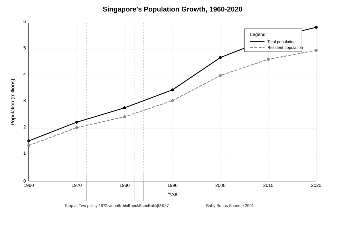
Study Figure 4, which shows Singapore's population growth from 1960 to 2020.
(a) State the total population of Singapore in 2010.
_______________________________________________ [1]
(b) Calculate the percentage growth in total population between 1990 and 2010. Give your answer to one decimal place. Show your working.
_______________________________________________
_______________________________________________
_______________________________________________ [3]
(c) Describe the trend in the gap between total population and resident population from 1960 to 2020.
_______________________________________________
_______________________________________________
_______________________________________________ [2]
(d) Suggest one reason why the gap between total population and resident population increased after 2000.
_______________________________________________
_______________________________________________ [2]
7.
Generated graph for Q7.
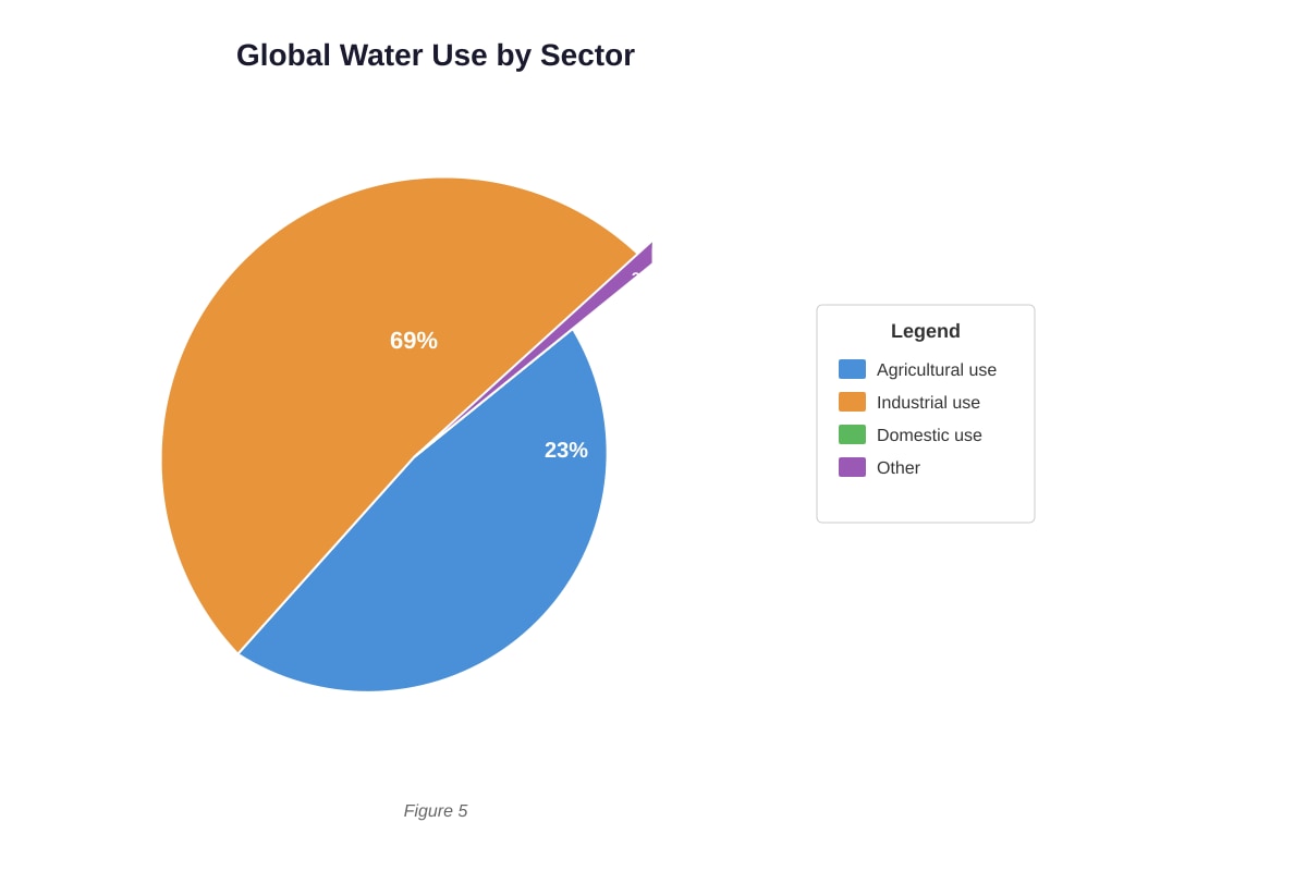
Study Figure 5, which shows global water use by sector.
(a) State the percentage of global water used for agricultural purposes.
_______________________________________________ [1]
(b) Calculate the ratio of industrial water use to domestic water use. Give your answer in its simplest form.
_______________________________________________
_______________________________________________ [2]
(c) Explain why agriculture requires a larger proportion of global water use compared to domestic use.
_______________________________________________
_______________________________________________
_______________________________________________ [3]
8.
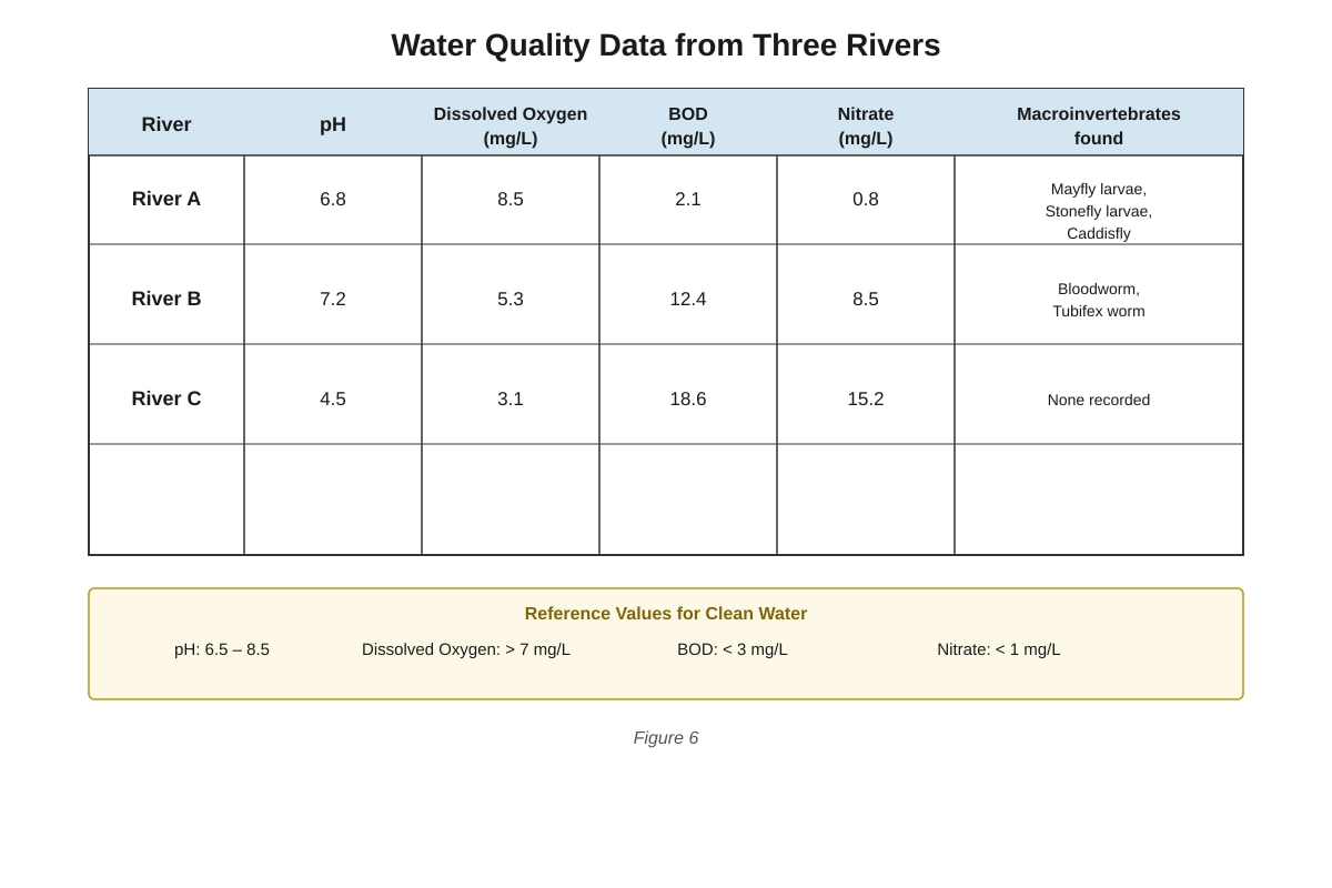
Generated table for Q8.
Study Figure 6, which presents water quality data from three rivers.
(a) Using the reference values provided, identify which river has the best overall water quality. Give two pieces of evidence from the data to support your answer.
River: _________________________________________
Evidence 1: _____________________________________
Evidence 2: _____________________________________ [3]
(b) River C has no macroinvertebrates recorded. Explain what this indicates about the water quality of River C.
_______________________________________________
_______________________________________________
_______________________________________________ [2]
(c) Suggest one possible human activity that could cause the high nitrate levels in River C.
_______________________________________________
_______________________________________________ [2]
Section B Total: 24 marks
Section C: Data Analysis, Evaluation and Geographical Inquiry
Total: 16 marks | Suggested time: 20 minutes
9.
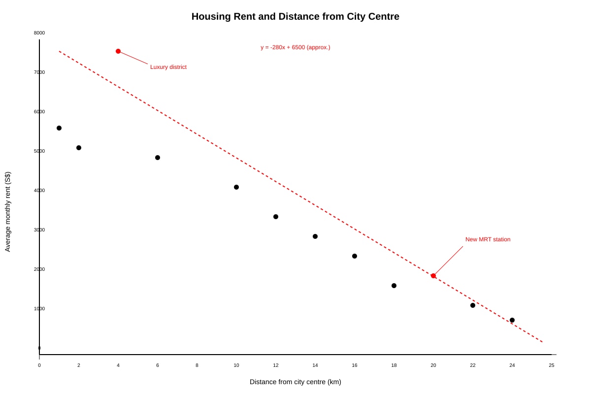
Generated graph for Q9.
Study Figure 7, a scatter graph showing the relationship between distance from city centre and average monthly housing rent.
(a) Describe the general relationship shown by the line of best fit.
_______________________________________________
_______________________________________________ [2]
(b) Using the line of best fit, estimate the average monthly rent for a property 14 km from the city centre. Show your working on the graph or below.
_______________________________________________
_______________________________________________ [2]
(c) Explain why the data point at 3 km, labelled "Luxury district," does not follow the general pattern.
_______________________________________________
_______________________________________________
_______________________________________________ [2]
(d) The data point at 20 km is labelled "New MRT station." Explain how a new MRT station could cause rent to be higher than expected at this distance.
_______________________________________________
_______________________________________________
_______________________________________________ [3]
10. A group of Secondary 1 students planned a fieldwork investigation to compare water quality in two streams: one flowing through a forested area (Stream X) and one flowing through an urban estate with many houses (Stream Y).
(a) State one hypothesis the students could test in this investigation.
_______________________________________________ [1]
(b) Identify two pieces of equipment the students would need to collect water quality data, and state what each piece of equipment would measure.
Equipment 1: ____________________________________
Measures: _____________________________________
Equipment 2: ____________________________________
Measures: _____________________________________ [4]
(c) Explain two safety precautions the students should take when working near the streams.
Precaution 1: ___________________________________
Reason: _______________________________________
Precaution 2: ___________________________________
Reason: _______________________________________ [4]
(d) Suggest one way the students could make their results more reliable.
_______________________________________________
_______________________________________________ [2]
11.
Image pending generation: graph for Q11.
Study Figure 8, a climate graph for a tropical rainforest location.
(a) Calculate the annual temperature range shown in the graph. Show your working.
_______________________________________________
_______________________________________________ [2]
(b) Explain why tropical rainforest locations have a small annual temperature range.
_______________________________________________
_______________________________________________
_______________________________________________ [3]
(c) Compare the reliability of the climate data in Figure 8 with data collected by the students in Question 10 during a single day of fieldwork.
_______________________________________________
_______________________________________________
_______________________________________________ [2]
Section C Total: 16 marks
END OF PAPER
Total Marks: 60
Extra Space
If you need extra space for any answer, write the question number clearly and continue below.
This practice paper was generated by TuitionGoWhere AI as syllabus-aligned practice material. It is not an official examination paper.
Answers
TuitionGoWhere Practice Paper - Geography Secondary 1
Answer Key and Marking Scheme
Version: 2 of 5
Section A: Map Skills and Spatial Data
Total: 20 marks
Question 1
(a) State the 4-figure grid reference of the settlement of Baymouth.
Answer: 3463 [1]
Teaching note: A 4-figure grid reference identifies a 1 km × 1 km square. Always read eastings (along the bottom or top) first, then northings (up the side). Baymouth is located where easting 34 meets northing 63, so the grid square is 3463. Common error: writing 6334 (reversing the order) — always remember "along the corridor, then up the stairs."
(b) State the 6-figure grid reference of the spot height 156 m.
Answer: 338664 [1]
Teaching note: A 6-figure grid reference pinpoints a location to within 100 m. The easting 338 means 33.8 (between grid lines 33 and 34, about 8-tenths across). The northing 664 means 66.4 (between grid lines 66 and 67, about 4-tenths up). Common error: estimating position incorrectly — imagine each grid square divided into 10 equal parts vertically and horizontally.
(c) In which compass direction does the River Devin flow? Explain how you determined this.
Answer: West to east / from west towards east (accept: flows eastwards) [1]
Explanation: The river flows from higher land to lower land / contours show higher ground (156 m) in the west and lower ground near the coast in the east / rivers flow downhill and contour lines bend uphill where they cross a river (V-shape points upstream) [1]
Teaching note: Rivers always flow from higher elevation to lower elevation. On topographic maps, contour lines form a V-shape when crossing a river, with the V pointing upstream (towards the source). The 156 m spot height in the western part of the map and the river reaching sea level at the coast confirm the direction. Alternative method: use the north arrow and observe the general downhill trend from west to east.
(d) Calculate the straight-line distance, in kilometres, between the spot height 45 m and the spot height 102 m. Show your working.
Answer: Working shown: approximately 2.4 km (accept 2.3–2.5 km) [3]
Step-by-step working:
- Step 1: Measure the map distance between the two spot heights using a ruler [1]
(Expected measurement: approximately 9.6 cm, but accept reasonable variation due to reproduction) - Step 2: Use the scale: 1:25 000 means 1 cm on map = 25 000 cm on ground = 0.25 km [1]
Concept: Scale converts map distances to real-world distances. 25 000 cm = 250 m = 0.25 km. - Step 3: Calculate: 9.6 cm × 0.25 km/cm = 2.4 km [1]
Teaching note: The scale 1:25 000 is a representative fraction. It means 1 unit on the map represents 25 000 of the same units on the ground. To convert: 25 000 cm = 250 m = 0.25 km. Therefore, multiply any centimetre measurement by 0.25 to get kilometres. Common error: forgetting to convert cm to km correctly — 25 000 cm is 0.25 km, not 25 km.
(e) Describe the relief (shape of the land) in grid square 3466.
Answer: Gentle slope / sloping land / rising ground [1] with elaboration: contours are spaced fairly far apart indicating gradual change in height / land rises from southeast to northwest (or specified direction) [1]
Teaching note: Relief description requires interpreting contour spacing. Close contours = steep slope; widely spaced contours = gentle slope. In grid square 3466, contours should be relatively widely spaced (based on map design), indicating a gentle slope. You should also identify the direction of slope by reading contour values — higher numbers indicate higher ground.
Question 2
(a) Identify the type of road shown by the symbol at grid reference 3364.
Answer: Main road / secondary road / B-road (accept: Road B542) [1]
Teaching note: On Ordnance Survey style maps, roads are shown with different symbols: motorways (blue with stripes), A-roads (red), B-roads (orange/brown), minor roads (yellow/white). The reference to "B542" in the map labels indicates this is a B-class road, a secondary road.
(b) Name the human feature found at 6-figure grid reference 338663.
Answer: Lighthouse [1]
Teaching note: The 6-figure reference 338663 (easting 338, northing 663) places this location at the coastal point where the lighthouse symbol should be positioned based on the map description. Always read eastings first: 338 is between grid lines 33 and 34, 8-tenths across. Northing 663 is between grid lines 66 and 67, 3-tenths up.
(c) Suggest one reason why the railway line was built along its current route rather than taking a more direct path across the higher land.
Answer: Any one valid reason: [2]
- To avoid steep gradients: Railway engines struggle to climb steep slopes / it is easier and cheaper to build on gentler land [1], so following lower ground around hills reduces the gradient [1]
- To follow the valley: The river valley provides a natural route with gentler slopes [1], reducing need for cuttings and tunnels [1]
- Cost: Cutting through higher land would require tunnels and expensive engineering works [1], following the coast/lower land is cheaper [1]
- Settlements: The route passes through or near settlements to serve passengers and freight [1], linking Baymouth to other communities [1]
Teaching note: Engineers choose routes that balance cost, engineering feasibility, and service to population. Railways need gradients typically below 1:100 (1 m rise per 100 m forward) for efficiency. Contour lines show that direct routes over higher ground would cross closely spaced contours (steep slopes), requiring expensive earthworks or tunnels.
Question 3
(a) What is the total length of the walking trail from Car Park A to Lighthouse Point?
Answer: 10 km [1]
Teaching note: Direct reading from the map — distance markers every 2 km show 10 km total at the end point.
(b) Calculate the horizontal equivalent distance on the ground, in metres, represented by 2 cm on this map. Show your working.
Answer: 1000 m / 1 km [2]
Working:
- Step 1: Scale 1:50 000 means 1 cm on map = 50 000 cm on ground [1]
- Step 2: 2 cm on map = 2 × 50 000 cm = 100 000 cm = 1000 m (or 1 km) [1]
Teaching note: The scale 1:50 000 means each centimetre represents 50 000 centimetres in reality. 50 000 cm = 500 m = 0.5 km. For 2 cm: 2 × 0.5 km = 1 km = 1000 m. Two-step process: (1) find what 1 cm represents, (2) multiply by the measured centimetres.
(c) A walker completes the trail in 3 hours. Calculate the average walking speed in km/h.
Answer: 3.3 km/h (accept 3⅓ km/h) [2]
Working:
- Step 1: Formula: Speed = Distance ÷ Time [1]
- Step 2: Speed = 10 km ÷ 3 hours = 3.333... km/h ≈ 3.3 km/h [1]
Teaching note: Speed calculations always use distance divided by time. Units must match — if distance is in km and time in hours, speed is in km/h. For exact answer: 10/3 = 3.333... which rounds to 3.3 km/h (1 decimal place) or can be left as 3⅓ km/h. Common error: dividing time by distance (3 ÷ 10 = 0.3) — always put distance on top.
Question 4
(a) Describe the elevation pattern along the trail from start to finish.
Answer: Any valid description covering pattern: [2]
- General trend: Starts at low elevation (0-50 m, dark green) [1], generally increases to highest point (over 200 m, brown zone) [1], then decreases towards the end at Lighthouse Point (coastal, back to low elevation) [1]
- Maximum two marks: Must describe both overall increase and subsequent decrease, or describe progressive zones
Teaching note: "Describe" requires identifying patterns, not just listing numbers. The colour bands indicate: dark green = 0-50 m (low), light green = 51-100 m (moderate), yellow = 101-200 m (high), brown = 201+ m (very high). The trail starts low, climbs through all zones to maximum height, then descends to coastal lighthouse.
(b) Explain why the final 2 km of the trail might be the most challenging section for walkers.
Answer: [2]
- Steep descent: The final section drops from yellow/brown zone (high elevation) to sea level (0 m) in only 2 km [1], meaning a steep gradient / rapid height loss [1]
- Cliff terrain: The cliff symbol indicates dangerous drops / unstable ground [1], requiring careful navigation [1]
- Combined factors: Rapid descent plus uneven cliff terrain makes this section hazardous [2]
Teaching note: Gradient = vertical change ÷ horizontal distance. Dropping from ~220 m to 0 m in 2 km gives a gradient of 220/2000 = 11% or about 1:9, which is steep for walking. Cliff symbols on maps show where land drops sharply — these are physically demanding and potentially dangerous sections requiring caution.
Section A Total: 20 marks
Section B: Graph and Data Interpretation
Total: 24 marks
Question 5
(a) State the total rainfall, in mm, for the month of November.
Answer: 240 mm (accept 235–245 mm range due to graph reading) [1]
Teaching note: Read directly from the compound bar graph. November's total bar height should reach approximately 240 mm on the left Y-axis. Use a ruler or straight edge to align the top of the bar with the scale. The bar is divided into components, but the question asks for total height.
(b) Identify the wettest three-month period and the driest three-month period.
Answer: [2]
- Wettest: November–December–January (accept Oct–Nov–Dec or Nov–Jan) [1]
- Driest: June–July–August (accept May–Jun–Jul or Jun–Aug) [1]
Teaching note: For "wettest," look for the three consecutive months with highest combined totals. Nov (240) + Dec (280) + Jan (220) = 740 mm, or using Oct (190) instead of Jan = 710 mm. Either grouping is valid as both are clearly wetter than other periods. For "driest," Jun (130) + Jul (160) + Aug (170) = 460 mm is clearly lowest. "Consecutive" means following one after another without gaps.
(c) Describe the relationship between temperature and convectional rainfall shown in the graph. Use evidence from the data.
Answer: [3]
Positive relationship/correlation identified: Higher temperatures are associated with higher convectional rainfall [1]
Evidence:
- Months with temperatures above 27.5°C (April–September) have substantial convectional rainfall components [1]
- Example: May has temperature ~27.8°C with high convectional rainfall; January has lower temperature ~26.0°C with minimal convectional rainfall [1]
Teaching note: Convectional rainfall occurs when intense heating causes air to rise rapidly, cool, and condense into rain. Singapore's position near the equator means year-round heating, but afternoon convection is strongest when temperatures peak. The graph shows convectional rain dominates March–October when temperatures are slightly higher, while monsoonal rain dominates "cooler" months (still hot by global standards, but relatively cooler).
(d) Explain why Singapore experiences convectional rainfall mainly in the afternoon.
Answer: [3]
Heating process:
- The sun heats the ground and buildings strongly throughout the morning [1]
- Air in contact with the heated surfaces warms and becomes less dense [1]
- Warm, moist air rises rapidly in convection currents [1]
- As rising air cools to dew point, water vapour condenses into cumulonimbus clouds [1]
- Heavy afternoon thunderstorms result [1]
Maximum 3 marks — any three valid points from above
Teaching note: This is the classic convection process. Key geographical concept: intense insolation (solar heating) near the equator creates strong convection. The daily cycle matters — morning heating accumulates, peak convection occurs early-to-mid afternoon when surface temperatures are highest. Cumulonimbus clouds produce heavy but short-lived rainfall. Singapore's location 1°N of equator means this mechanism operates year-round but varies in intensity with the seasons.
Question 6
(a) State the total population of Singapore in 2010.
Answer: 5.1 million (accept 5.08–5.15 million) [1]
Teaching note: Direct reading from the line graph — locate 2010 on X-axis, move vertically to the solid line (total population), read across to Y-axis.
(b) Calculate the percentage growth in total population between 1990 and 2010. Give your answer to one decimal place. Show your working.
Answer: 70.0% [3]
Step-by-step working:
- Step 1: Identify values: 1990 = 3.0 million; 2010 = 5.1 million [1]
- Step 2: Calculate increase: 5.1 − 3.0 = 2.1 million [1]
(or: percentage growth = [(new − old) ÷ old] × 100) - Step 3: [(2.1 ÷ 3.0) × 100] = (0.7 × 100) = 70.0% [1]
Teaching note: Percentage change formula is always: [(New Value − Original Value) ÷ Original Value] × 100. The original value (1990) is the base for comparison. Common errors: using 5.1 as denominator; forgetting to multiply by 100; calculation errors. Show all steps clearly for method marks.
(c) Describe the trend in the gap between total population and resident population from 1960 to 2020.
Answer: [2]
- The gap increases / widens / grows over time [1]
- Evidence of acceleration: Gap was small in 1960 (0.1 million), moderate in 1990 (0.3 million), then larger in 2000 (0.7 million), 2010 (1.3 million), and 2020 (1.7 million) — accept any specific data comparison showing increase [1]
Teaching note: The "gap" represents non-resident population (work permit holders, dependents, etc.). Read both lines for each year and subtract: 1960: 1.6−1.5=0.1; 1970: 2.0−1.9=0.1; 1980: 2.4−2.2=0.2; 1990: 3.0−2.7=0.3; 2000: 4.0−3.3=0.7; 2010: 5.1−3.8=1.3; 2020: 5.7−4.0=1.7. The gap widens dramatically after 1990.
(d) Suggest one reason why the gap between total population and resident population increased after 2000.
Answer: Any one valid reason with development: [2]
- Foreign workers: More work permit holders employed in construction, domestic work, and services [1], attracted by economic growth and labour shortages [1]
- Global talent attraction: Policies to attract skilled professionals and investors [1], increasing Employment Pass and S-Pass holders [1]
- Dependency: Families of foreign workers / dependants joining workers [1], expanding non-resident numbers [1]
Teaching note: Singapore's economic growth strategy relied on imported labour at various skill levels. The "foreign workforce" policy expanded significantly in the 2000s. Students should connect economic policy to demographic data — the gap is a deliberate policy outcome, not merely accidental.
Question 7
(a) State the percentage of global water used for agricultural purposes.
Answer: 69% [1]
Teaching note: Direct reading from pie chart — the agricultural sector occupies the largest segment, clearly labelled 69%.
(b) Calculate the ratio of industrial water use to domestic water use. Give your answer in its simplest form.
Answer: 23:6 or approximately 3.83:1 or 23/6 [2]
Working:
- Industrial = 23%; Domestic = 6% [1]
- Ratio = 23:6 (this is already in simplest form as 23 is prime and does not divide by 2 or 3) [1]
Teaching note: A ratio compares two quantities in the same units. Here both are percentages, so the ratio is direct: 23:6. To simplify, find highest common factor (HCF). HCF of 23 and 6 is 1, so 23:6 is simplest form. Common error: writing as 23/6 without clarifying it's a ratio, or incorrectly "simplifying" to incorrect values.
(c) Explain why agriculture requires a larger proportion of global water use compared to domestic use.
Answer: [3]
Scale and process reasons:
- Large land area: Agriculture covers vast areas of land globally / farmland exceeds urban areas [1], requiring water across extensive regions [1]
- Evapotranspiration: Crops lose water through evaporation from soil and transpiration from plants [1], this combined loss is substantial [1]
- Irrigation needs: Many farming regions have insufficient rainfall / arid and semi-arid areas need artificial watering [1], adding to water demand [1]
- Food production: Agriculture feeds billions of people / water is essential for plant growth and productivity [1]
Maximum 3 marks — any three valid points with development
Teaching note: The 69% figure reflects that agriculture is fundamentally a water-intensive activity at global scale. Key concept: evapotranspiration. Plants need water not just for growth but to maintain structure (turgor pressure). In dry regions, irrigation multiplies water use. Domestic use (drinking, washing, cleaning) is small per person and concentrated in smaller areas.
Question 8
(a) Using the reference values provided, identify which river has the best overall water quality. Give two pieces of evidence from the data to support your answer.
Answer: [3]
River: River A [1]
Evidence (any two from):
- Dissolved Oxygen: 8.5 mg/L — exceeds the reference ">7 mg/L" for clean water / higher than Rivers B and C [1]
- BOD: 2.1 mg/L — below reference "<3 mg/L" / much lower than polluted rivers [1]
- Nitrate: 0.8 mg/L — below reference "<1 mg/L" / close to natural levels [1]
- pH: 6.8 — within clean water range (6.5–8.5) [1]
- Macroinvertebrates: Presence of mayfly, stonefly, caddisfly larvae — these are sensitive species that only thrive in clean water (bioindicators) [1]
Teaching note: Water quality assessment uses multiple indicators. Dissolved Oxygen (DO) is critical — aquatic life needs oxygen; high DO means water can support organisms. BOD (Biochemical Oxygen Demand) measures organic pollution — high BOD means bacteria are consuming oxygen faster than it's replaced. Mayfly and stonefly larvae are particularly sensitive to pollution; their presence is excellent evidence of clean water. River A meets all reference criteria; River B fails DO, BOD, and nitrate; River C fails all criteria severely.
(b) River C has no macroinvertebrates recorded. Explain what this indicates about the water quality of River C.
Answer: [2]
- Severe pollution / extremely poor water quality [1]
- Explanation: Macroinvertebrates are bioindicators / sensitive species cannot survive in polluted conditions [1], their absence indicates toxic levels of pollutants or extremely low oxygen [1]
Teaching note: Biological monitoring uses organism presence/absence as pollution indicators. Different species have different tolerances. Mayflies (EPT group: Ephemeroptera, Plecoptera, Trichoptera) are most sensitive. Bloodworms (midge larvae) tolerate moderate pollution. Tubifex worms tolerate severe organic pollution. Complete absence suggests conditions too harsh even for tolerant species — likely from extreme pH (4.5 is acidic, suggesting acid rain or industrial discharge), very low oxygen (3.1 mg/L), or toxic substances.
(c) Suggest one possible human activity that could cause the high nitrate levels in River C.
Answer: Any one valid with development: [2]
- Agriculture / fertiliser use: Farmers apply nitrogen-based fertilisers to crops [1], rain washes excess nitrates into rivers (runoff/leaching) [1]
- Livestock farming: Animal waste/manure contains high nitrogen levels [1], enters water through runoff or seepage [1]
- Sewage/ wastewater: Untreated or poorly treated sewage contains organic nitrogen [1], effluent discharge raises nitrate levels [1]
- Industrial discharge: Factories releasing nitrogen-rich waste [1], direct pollution into waterways [1]
Teaching note: Nitrates are plant nutrients. Natural levels in unpolluted water are <1 mg/L. Elevated nitrates cause eutrophication — excessive algae growth, oxygen depletion when algae die and decompose, harming aquatic life. The 15.2 mg/L in River C is enormously elevated, suggesting multiple sources or concentrated point-source pollution.
Section B Total: 24 marks
Section C: Data Analysis, Evaluation and Geographical Inquiry
Total: 16 marks
Question 9
(a) Describe the general relationship shown by the line of best fit.
Answer: [2]
- Negative correlation / inverse relationship [1]
- Description: As distance from city centre increases, average monthly rent decreases [1] / rent is highest near the city centre and lowest farther away [1]
Teaching note: The line of best fit shows the general trend, ignoring outliers. Negative correlation means one variable increases while the other decreases. The downward slope (approximately −280 S/km)indicatesthateachkilometrefartherfromcentrereducesrentbyaboutS280 on average. This is the classic bid-rent theory pattern — land values peak at most accessible locations.
(b) Using the line of best fit, estimate the average monthly rent for a property 14 km from the city centre. Show your working on the graph or below.
Answer: Approximately S2580–S2 660 (accept range from line of best fit) [2]
Working using equation:
- y = −280x + 6 500 (approximate equation given) [1]
- When x = 14: y = (−280 × 14) + 6 500 = −3 920 + 6 500 = S$2 580 [1]
Alternative — graphical estimation:
- Locate 14 km on X-axis, move up to line of best fit, read across to Y-axis [1]
- Y-axis reading approximately S2600±S80 [1]
Teaching note: Two valid methods: (1) graphical estimation using the line of best fit, (2) calculation using the equation. The equation method is more precise. Common errors: using a data point instead of the line; incorrect reading of the Y-axis scale; arithmetic errors in substitution.
(c) Explain why the data point at 3 km, labelled "Luxury district," does not follow the general pattern.
Answer: [2]
- Location quality: The luxury district offers premium amenities / prestigious address / high-status neighbourhood [1]
- Demand factors: Wealthy buyers/renters are willing to pay premium prices for exclusivity, security, and quality [1]
- Non-distance factors: Other factors besides distance affect rent — landscaping, building quality, views, proximity to specific attractions [1]
Maximum 2 marks — any two valid developed points
Teaching note: Outliers indicate where other factors override the general pattern. Real estate markets are influenced by amenity, prestige, and neighbourhood effects (bid-rent theory modified by social factors). The luxury district may include embassy areas, protected heritage zones, or premium developments where scarcity and status create above-average prices.
(d) The data point at 20 km is labelled "New MRT station." Explain how a new MRT station could cause rent to be higher than expected at this distance.
Answer: [3]
Accessibility change:
- The MRT station improves public transport links to the city centre / reduces travel time [1]
- Previously distant location becomes well-connected / commute becomes convenient [1]
Demand increase:
- More people want to live near the MRT station / demand for housing increases [1]
- Higher demand pushes up prices and rents / scarcity of nearby housing [1]
Spatial restructuring:
- MRT creates a "node" of accessibility in the suburban area [1], local commercial development follows [1], increasing area desirability [1]
Maximum 3 marks — any three valid developed points
Teaching note: Transport infrastructure reshapes spatial patterns. Before MRT, 20 km distance meant poor access (long bus rides, traffic congestion). After MRT, door-to-door time to centre may be 30–35 minutes — comparable to some inner areas by road. This is "spatial convergence" or "time-space compression." The MRT creates a "transport advantage" that capitalises into land values. This is why public transport investment is a key planning tool.
Question 10
(a) State one hypothesis the students could test in this investigation.
Answer: Any one testable hypothesis: [1]
- "Stream X has better water quality than Stream Y"
- "Water in the forested stream has higher dissolved oxygen than water in the urban stream"
- "The urban stream has higher nitrate levels than the forested stream"
- "More macroinvertebrate species will be found in Stream X than Stream Y"
Teaching note: A hypothesis must be testable (can be investigated with data collection) and directional (predicts a relationship or difference). Avoid vague statements like "water quality is different" — specify what difference and in what direction. The hypothesis should relate to causes (forest vs urban land use) and measurable effects (water quality indicators).
(b) Identify two pieces of equipment the students would need to collect water quality data, and state what each piece of equipment would measure.
Answer: [4]
Equipment 1: pH meter / Universal Indicator paper / pH probe [1]
Measures: pH / acidity or alkalinity [1]
Equipment 2: Dissolved oxygen meter / DO probe / Winkler titration kit [1] — OR alternatives: thermometer (temperature), Secchi disk/tube (turbidity), nitrate test kit (nitrate concentration), sampling net (macroinvertebrates), GPS unit (location)
Measures: Dissolved oxygen concentration in mg/L [1]
Teaching note: Equipment must match measurable indicators. pH equipment measures hydrogen ion concentration (0–14 scale). DO meters use electrochemical sensors. Acceptable alternatives: thermometer (temperature affects oxygen solubility and biological activity), nitrate test kits (colorimetric comparison), kick sampling nets (for macroinvertebrate collection), GPS (for precise location recording). Each answer needs both equipment name AND what it measures.
(c) Explain two safety precautions the students should take when working near the streams.
Answer: [4]
Precaution 1: Wear rubber boots/waders / avoid going barefoot [1]
Reason: Protects against slippery rocks, broken glass, sharp objects, and waterborne diseases (e.g., leptospirosis from rat urine) [1]
Precaution 2: Never work alone / work in groups with teacher supervision [1]
Reason: Allows help if someone falls in, has an accident, or feels unwell / drowning risk or injury requires immediate assistance [1]
Alternative Precaution 2: Wash hands after handling water / use gloves
Reason: Prevents infection from contaminated water / some streams carry bacteria, parasites, or chemicals
Alternative Precaution 2: Be careful of river banks / do not lean over deep water
Reason: Banks may be undercut and unstable / risk of falling into deeper water
Teaching note: Fieldwork safety addresses specific hazards: slippery surfaces (wet rocks, algae), water depth/current, biological contamination, isolated locations. Best answers connect precaution to specific risk. Rubber boots are standard for stream work — they provide grip, protection, and some flotation assistance. Pair working is essential — lone working near water is prohibited in most school policies.
(d) Suggest one way the students could make their results more reliable.
Answer: Any one valid method with development: [2]
- Repeat measurements: Take multiple samples at each site (e.g., three readings at each stream) [1], calculate averages to reduce random errors / identify anomalous results [1]
- Standardised timing: Collect all samples at the same time of day [1], to control for daily variations in water quality / temperature and DO vary diurnally [1]
- Multiple sites: Sample several points along each stream [1], to account for variation within each stream / avoid atypical single points [1]
- Control variables: Use same equipment and method for both streams [1], ensures fair comparison / systematic differences don't affect results [1]
Teaching note: Reliability means consistency — would the same method produce similar results if repeated? It's different from validity (measuring what you intend) and accuracy (closeness to true value). In fieldwork, reliability is improved by repetition, standardisation, and controlling variables. For water quality, diurnal variation matters — morning and afternoon readings can differ due to temperature, photosynthesis (affecting oxygen), and human activity patterns.
Question 11
(a) Calculate the annual temperature range shown in the graph. Show your working.
Answer: 2°C (accept 1.5–2.5°C depending on graph reading) [2]
Working:
- Step 1: Identify highest mean monthly temperature ≈ 28°C (May/June) [1]
Identify lowest mean monthly temperature ≈ 26°C (January/December) - Step 2: Annual range = 28 − 26 = 2°C [1]
Teaching note: Annual temperature range = highest monthly mean − lowest monthly mean. Do not use daily extremes. For tropical rainforest climate, the range is very small — characteristic of equatorial locations where insolation is consistent year-round. Compare with temperate climates where ranges of 15–25°C are common. The small range is a defining feature that students must calculate and explain.
(b) Explain why tropical rainforest locations have a small annual temperature range.
Answer: [3]
Solar angle consistency:
- The location is near the equator (low latitude) [1]
- The sun's rays strike at a high angle all year / overhead at equinoxes [1]
- Day length varies little — approximately 12 hours throughout the year [1]
Atmospheric processes:
- High cloud cover and humidity moderate temperatures [1], clouds reflect solar radiation by day and trap heat by night [1]
- High evapotranspiration from dense vegetation uses energy, limiting temperature rise [1]
Maximum 3 marks — any three valid developed points
Teaching note: Core concept: solar geometry. At the equator, the sun is always high in the sky (altitude > 60° even at midday in "winter"). This means consistent energy input. Contrast with mid-latitudes where winter sun is low angle, oblique rays spread over larger area, and days are short. The "thermal equator" concept — temperatures stay within narrow band because there's no "summer" or "winter" in the conventional sense, just wetter or drier periods.
(c) Compare the reliability of the climate data in Figure 8 with data collected by the students in Question 10 during a single day of fieldwork.
Answer: [2]
Climate graph (Figure 8):
- More reliable / highly reliable [1]
- Based on long-term averages (typically 30 years of data) / many years of measurements / reduces impact of unusual weather in single years [1]
Student fieldwork data:
- Less reliable / limited reliability [1]
- Single day only / short-term snapshot / may capture unusual conditions not representative of normal stream quality / no repetition to check consistency [1]
Maximum 2 marks — comparison point about Figure 8's reliability [1], contrast with students' data limitations [1]
Teaching note: climatological normals use 30-year averages (WMO standard). Single-day fieldwork captures one moment — weather may be atypical, water quality may vary with recent rainfall, time of day matters. Reliability increases with temporal and spatial sampling. Students should recognise that their single investigation provides useful but limited data; repeated visits, different times of year, and multiple years would improve reliability.
Section C Total: 16 marks
Grand Total: 60 marks
This answer key was generated by TuitionGoWhere AI as syllabus-aligned practice material. It is not derived from official examination marking schemes.
Free quiz and exam paper access
Enter your details to view this paper
Your access is remembered on this device.