From Real Exams Exam Paper

Secondary 1 Geography Semestral Assessment 2 (End of Year) Paper 4

Free Sec 1 Geography SA2 Paper 4, HY3 Exam version, with questions, answers, and syllabus-aligned practice for Singapore students.

These static practice materials are generated from the site's syllabus and paper-generation workflow, with source and model context shown so students and parents can evaluate the material before use.

Secondary 1 Geography From Real Exams Generated by Tencent HY3 Free Updated 2026-08-17

Back to Subject Browse Free Exam Papers

Questions

TuitionGoWhere Exam Practice (AI) — SA2 Geography Secondary 1

School: TuitionGoWhere Secondary School (AI)
Subject: Geography
Level: Secondary 1
Paper: SA2 Practice Paper (Version 4 of 5)
Duration: 60 minutes
Total Marks: 60
Name: ___________________________
Class: ________
Date: ____________

Instructions:

Answer all questions in the spaces provided.
Use a 2B pencil for any shading; use blue/black pen for writing.
Read each question carefully and study the figures, maps, and tables before answering.
Marks for each question are shown in brackets [ ].
Section totals and question marks add up to 60.

Section A: Map Reading (20 marks)

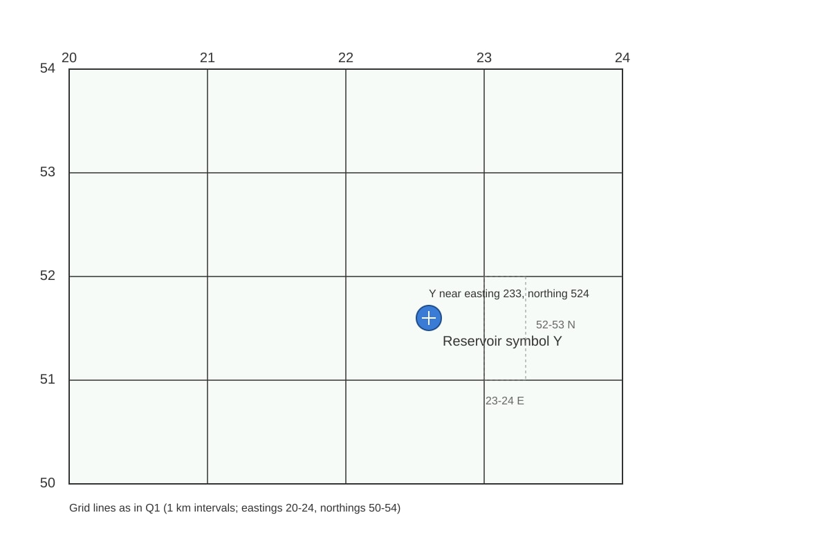
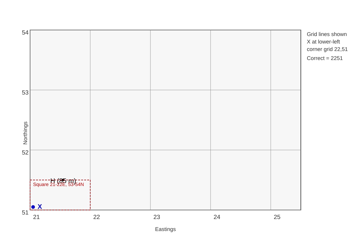
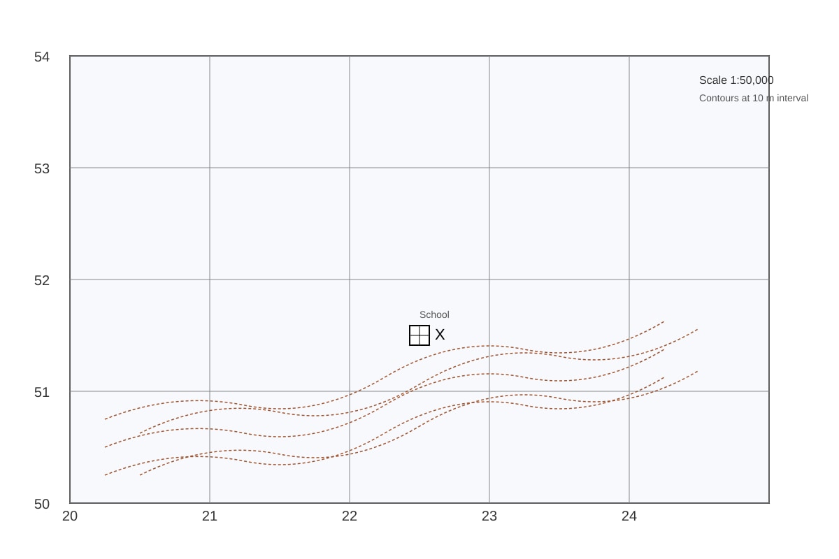
1. Study the map extract below. State the four-figure grid reference of the school labelled X. [1]

Map for Q1 (SEC1 Geography)

Generated map for Q1.

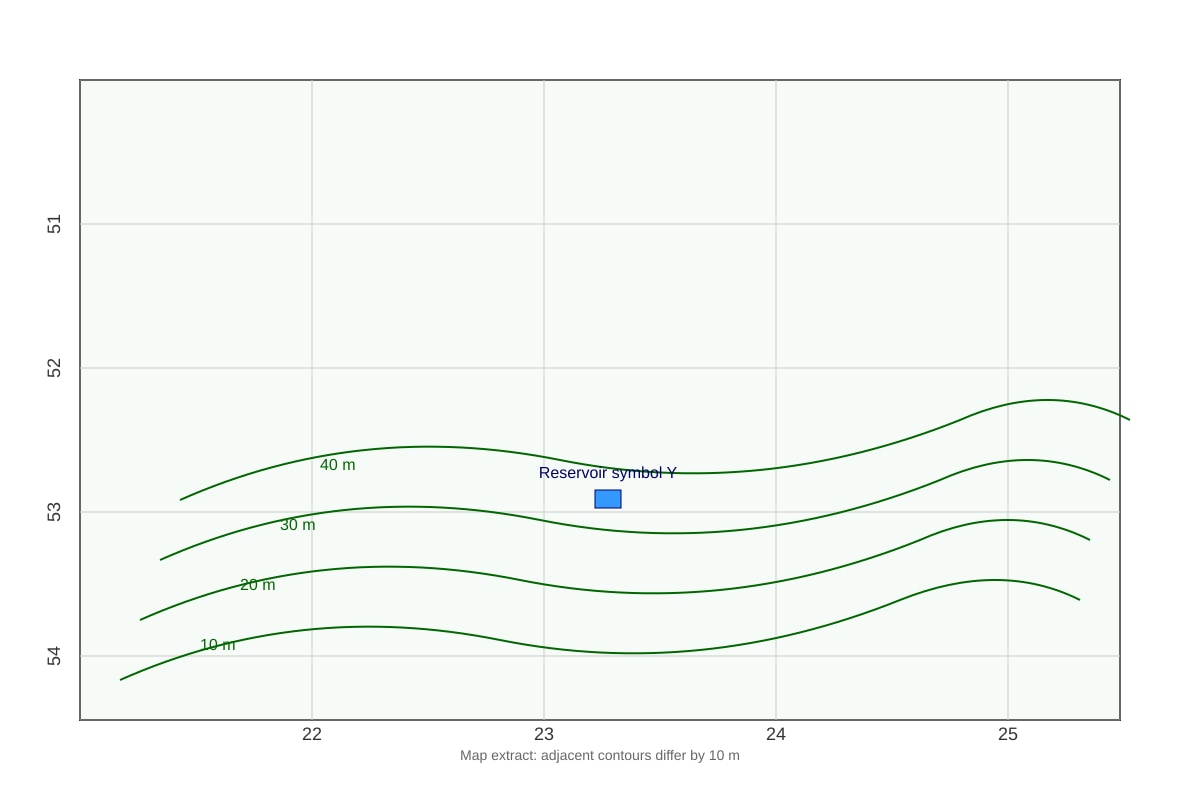
2. State the six-figure grid reference of the reservoir labelled Y on the same map extract. [1]

Map for Q2 (SEC1 Geography)

Generated map for Q2.

3. State the contour interval of the map extract. [1]

Map for Q3 (SEC1 Geography)

Generated map for Q3.

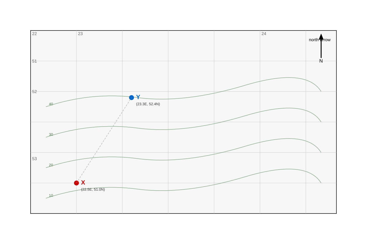
4. Give the bearing from the school X to the reservoir Y. [2]

Map for Q4 (SEC1 Geography)

Generated map for Q4.

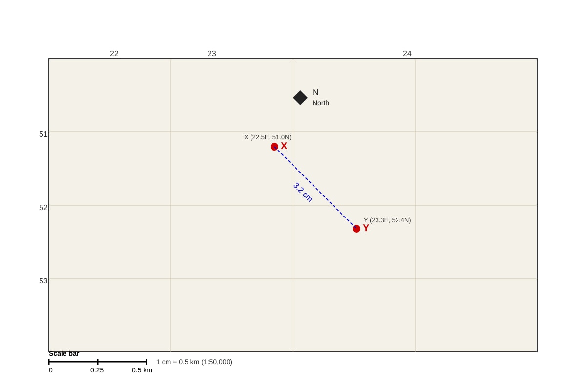
5. Calculate the straight-line distance, in km, from X to Y using the map scale 1:50,000. [2]

Map for Q5 (SEC1 Geography)

Generated map for Q5.

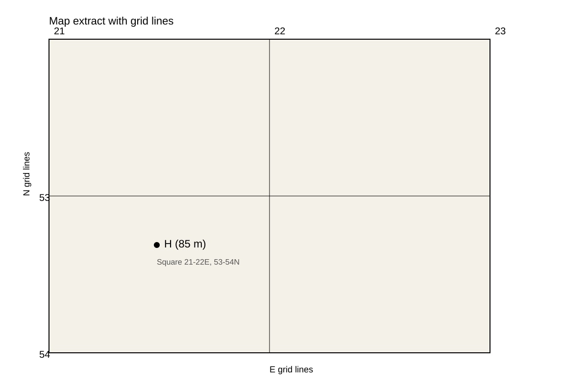
6. State the four-figure grid reference of the highest point marked H on the map. [1]

Map for Q6 (SEC1 Geography)

Generated map for Q6.

7. Describe one difference between a 4-figure and a 6-figure grid reference. [2]

8. A student says the grid reference of X is 5122. Explain the mistake. [2]

Map for Q8 (SEC1 Geography)

Generated map for Q8.

9. State the map scale as a ratio from the scale bar. [1]

Map for Q9 (SEC1 Geography)

Generated map for Q9.

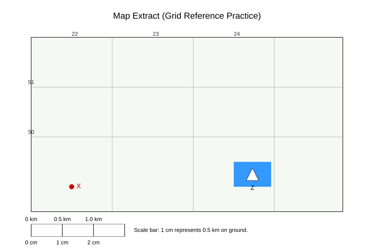
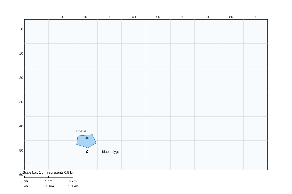
10. Identify the land use shown by the symbol Z (triangle inside blue area). [2]

Map for Q10 (SEC1 Geography)

Generated map for Q10.

Section B: Graph & Table Interpretation (20 marks)

11. Study the table below showing rainfall in mm for five towns. State the town with the highest rainfall. [1]

Town	Rainfall (mm)
A	120
B	205
C	98
D	176
E	150

12. Using the table in Q11, calculate the mean rainfall. [2]

13. Describe the pattern of rainfall across the five towns. [3]

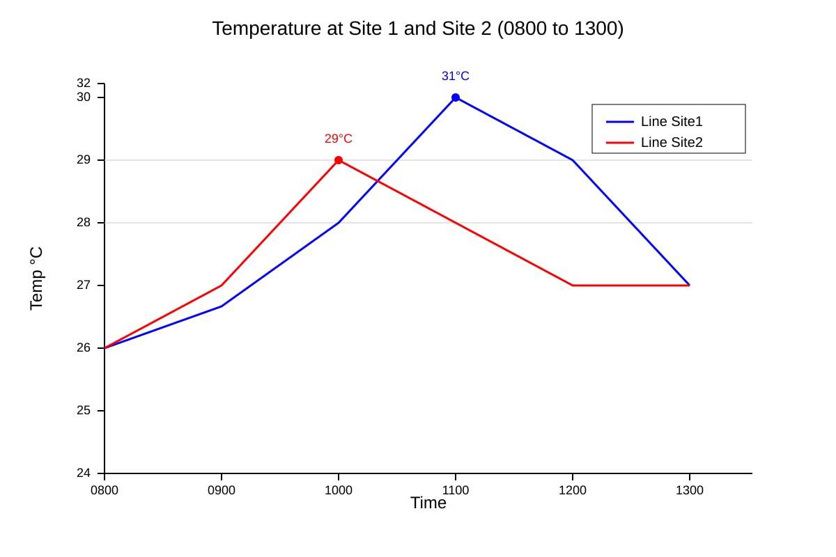
14. Study the line graph of temperature at Site 1 and Site 2 over 6 hours. State the time when Site 1 was warmest. [1]

Graph for Q14 (SEC1 Geography)

Generated graph for Q14.

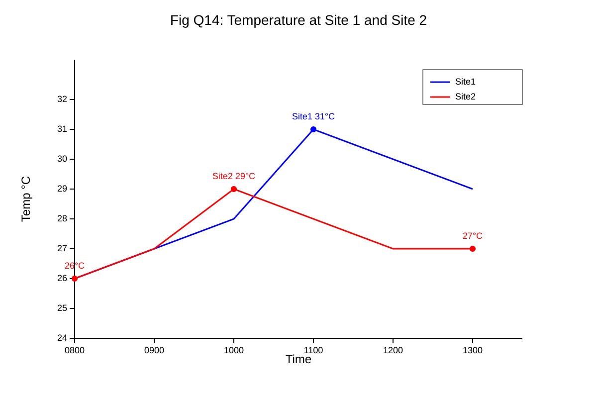
15. With reference to Fig Q14, describe how Site 2 temperature changed from 0800 to 1300. [3]

Graph for Q15 (SEC1 Geography)

Generated graph for Q15.

16. A bar chart shows forest area (% of land) for 4 countries: P 60, Q 35, R 12, S 5. State the country with smallest forest area. [1]

17. Calculate the range of forest area % from Q16. [2]

18. Explain why using a line graph for rainfall totals per month is suitable. [2]

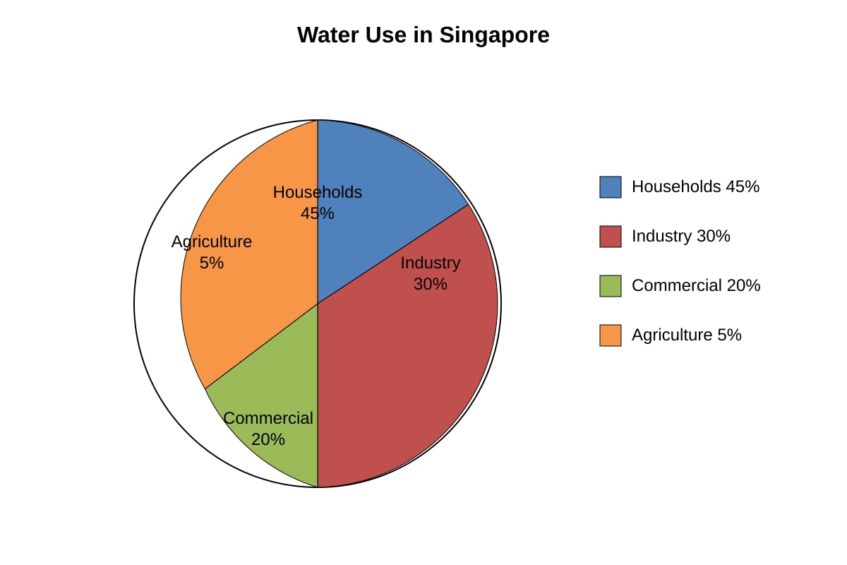
19. Study the pie chart of water use in Singapore. State the largest user category. [1]

Chart for Q19 (SEC1 Geography)

Generated chart for Q19.

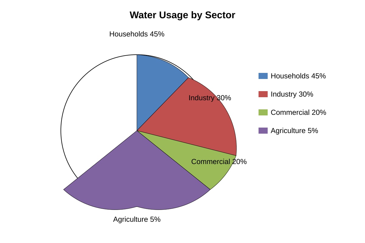
20. Using the pie chart in Q19, calculate the angle of the Industry slice. [2]

Chart for Q20 (SEC1 Geography)

Generated chart for Q20.

Section C: Data Skills Application (20 marks)

21. A class tested water quality at two sites. Table: Site A pH 7.2, DO 8 mg/L, turbidity 5 NTU; Site B pH 6.5, DO 4 mg/L, turbidity 20 NTU. State which site is healthier. [1]

22. Explain your answer to Q21 using two data values. [3]

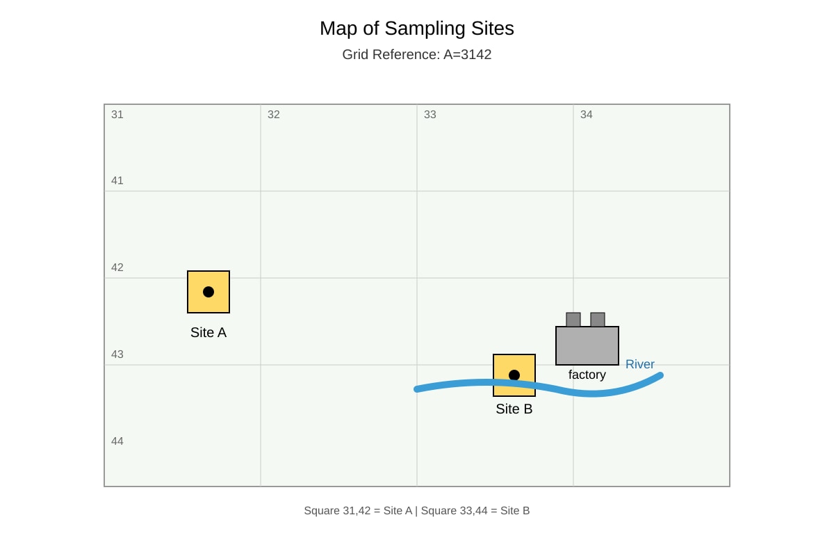
23. Study the map of the two sampling sites. Give the 4-figure grid ref of Site A. [1]

Map for Q23 (SEC1 Geography)

Generated map for Q23.

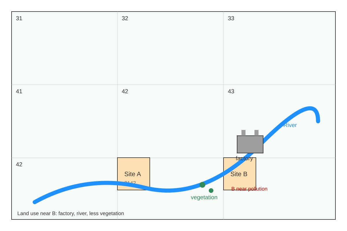
24. Suggest why Site B has higher turbidity. [2]

Map for Q24 (SEC1 Geography)

Generated map for Q24.

25. The table shows population (millions) of 3 cities in 2010 and 2020. Calculate % increase for City X (2.0 to 2.6). [2]

City	2010	2020
X	2.0	2.6
Y	1.5	1.8
Z	3.0	3.3

26. Describe the trend in population for all three cities. [3]

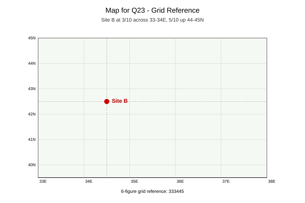
27. State the 6-figure grid reference of Site B from the map in Q23. [1]

Map for Q27 (SEC1 Geography)

Generated map for Q27.

28. A graph shows CO₂ emissions (tonnes) per year: 2015=10, 2018=14, 2021=18. Describe the trend. [3]

29. Calculate the total CO₂ emitted in the three years of Q28. [2]

30. Explain how a 6-figure grid reference improves map accuracy. [2]

31. State one advantage of showing data in a table rather than a paragraph. [1]

32. Using the rainfall table in Q11, what is the difference between Town B and Town C? [2]

33. A student draws a bar for Town A rainfall as 120 cm on a graph with y-axis in mm. State the error. [2]

34. With reference to the water quality table in Q21, state one reason pH below 7 may harm aquatic life. [2]

35. Give the bearing from Site A to Site B using the map in Q23. [2]

Map for Q35 (SEC1 Geography)

Generated map for Q35.

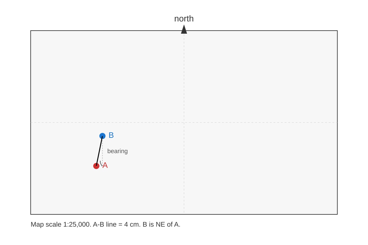
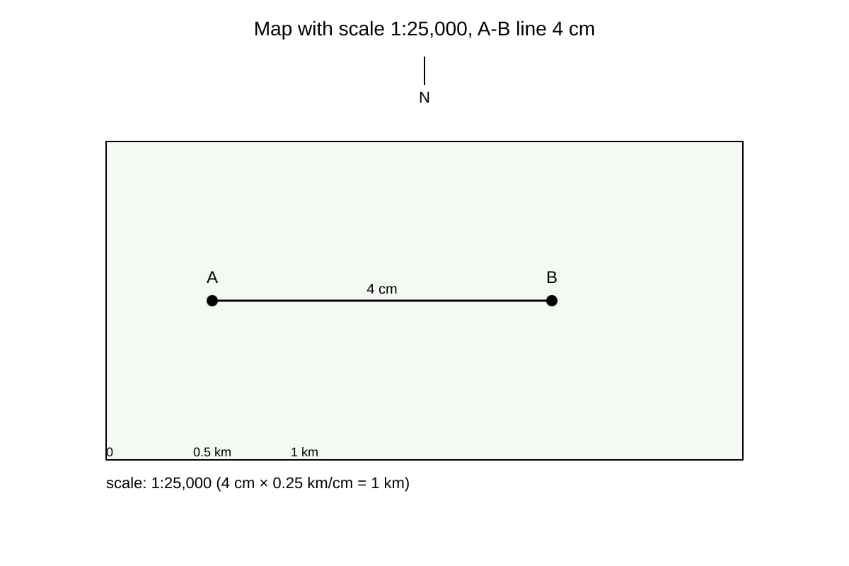
36. The map scale is 1:25,000. Site A to B measures 4 cm. Find ground distance in km. [2]

Map for Q36 (SEC1 Geography)

Generated map for Q36.

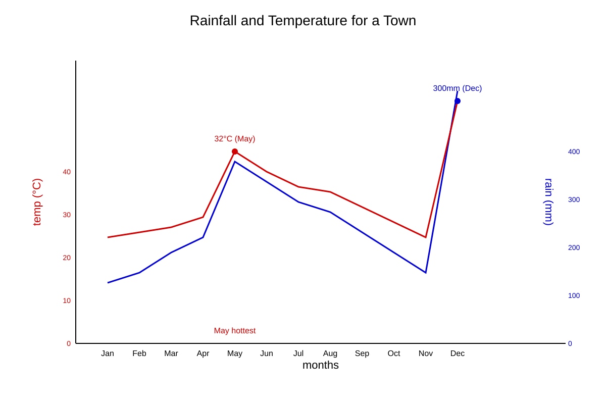
37. Study the graph of rainfall and temperature for a town (dual axis). State the month with highest temperature. [1]

Graph for Q37 (SEC1 Geography)

Generated graph for Q37.

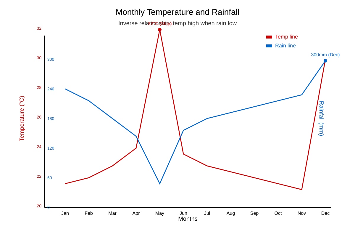
38. Describe the relationship between rainfall and temperature in Q37. [3]

Graph for Q38 (SEC1 Geography)

Generated graph for Q38.

39. A table shows forest loss (km²/yr): 2010=5, 2015=9, 2020=14. Calculate mean annual loss. [2]

40. Using all previous data, explain why geographers use both maps and graphs. [2]

Free quiz and exam paper access

Enter your details to view this paper

Your access is remembered on this device.

Answers

TuitionGoWhere Exam Practice (AI) — SA2 Geography Secondary 1 (Version 4) Answer Key

Total Marks: 60
Section A: 20, Section B: 20, Section C: 20 — adds to 60.

Section A: Map Reading

1. [1] 2251
Teaching: 4-figure grid reference = easting (across, left-to-right) first, then northing (up). X is in square with lower-left at 22 east, 51 north. Common mistake: writing 5122 (reversed).

2. [1] 233524 (acceptable 233524–233525)
Teaching: 6-figure = 4-figure + 3rd digit easting (tenths) + 3rd digit northing. Y at 233 east, 524 north. Estimate tenths from position in square.

3. [1] 10 m
Teaching: Contour interval = difference between adjacent labelled contours (20–10 = 10). Not map scale.

4. [2] Approximately 045° (north-east)
Teaching: Draw north line from X, measure angle to Y (NE direction). 1 mark direction, 1 mark reasonable bearing. Common: using south as up.

5. [2] 1.6 km
Working: Map dist = 3.2 cm. Scale 1:50,000 → 1 cm = 0.5 km. Ground = 3.2 × 0.5 = 1.6 km. Show substitution and unit.

6. [1] 2153
Teaching: H at square lower-left 21 east, 53 north.

7. [2] A 4-figure gives the grid square (100 m accuracy at 1:50k); a 6-figure gives a point within the square (100 m or better).
Marking: 1 mark each for accuracy and precision difference.

8. [2] Student reversed order (northing before easting). Correct is 2251.
Marking: 1 mark identify reversal, 1 mark correct reference.

9. [1] 1:50,000
Teaching: 1 cm = 0.5 km = 50,000 cm → ratio 1:50,000.

10. [2] Lake / reservoir (blue with triangle = dam or lake)
Marking: 1 mark water body, 1 mark specific symbol.

Section B: Graph & Table Interpretation

11. [1] Town B (205 mm)

12. [2] Mean = (120+205+98+176+150)/5 = 749/5 = 149.8 mm
Working shown; 1 mark sum, 1 mark division.

13. [3] Rainfall ranges from 98 mm (C) to 205 mm (B). B is highest, C lowest. General variation with no clear order.
Marking: 1 mark highest, 1 mark lowest, 1 mark overall pattern.

14. [1] 1100

15. [3] Site 2 rose from 26°C (0800) to 29°C (1000), then fell to 27°C (1300).
Marking: 1 mark rise, 1 mark peak, 1 mark fall.

16. [1] S (5%)

17. [2] Range = 60 – 5 = 55%
Working: max 60, min 5.

18. [2] Line graph shows change over time; rainfall per month is sequential so trend is clear.
Marking: 1 mark time suitability, 1 mark trend visibility.

19. [1] Households (45%)

20. [2] Angle = 30% × 360° = 108°
Working: full circle 360°, industry 30%.

Section C: Data Skills Application

21. [1] Site A

22. [3] Site A has higher DO (8 vs 4 mg/L) and lower turbidity (5 vs 20 NTU), so healthier.
Marking: 1 mark DO, 1 mark turbidity, 1 mark conclusion.

23. [1] 3142

24. [2] Factory near B releases silt; less vegetation to filter.
Marking: 1 mark pollution source, 1 mark vegetation.

25. [2] % increase = (2.6–2.0)/2.0 × 100 = 30%
Working shown.

26. [3] All three cities increased from 2010 to 2020 (X +0.6, Y +0.3, Z +0.3).
Marking: 1 mark all increase, 2 marks values.

27. [1] 333445 (approx)

28. [3] CO₂ rose steadily: 10 (2015) → 14 (2018) → 18 (2021).
Marking: 1 mark rise, 2 marks values.

29. [2] Total = 10+14+18 = 42 tonnes

30. [2] 6-figure locates a point within 100 m; 4-figure only square (1 km).
Marking: 1 mark point, 1 mark accuracy.

31. [1] Easy comparison of values.

32. [2] 205 – 98 = 107 mm

33. [2] Used cm instead of mm; bar should be 120 units not 120 cm.
Marking: 1 mark unit error, 1 mark correction.

34. [2] pH <7 is acidic; can stress or kill sensitive species.
Marking: 1 mark acidic, 1 mark harm.

35. [2] Approximately 045° (NE)
Marking: direction from A to B.

36. [2] 4 cm × 0.25 km/cm = 1.0 km
Scale 1:25,000 → 1 cm = 0.25 km.

37. [1] May

38. [3] Temperature high when rainfall low (inverse); May hot & dry, Dec cool & wet.
Marking: 1 mark inverse, 2 marks examples.

39. [2] Mean = (5+9+14)/3 = 9.33 km²/yr

40. [2] Maps show location/space; graphs show change/trend. Both needed for full analysis.
Marking: 1 mark each.