From Real Exams Quiz

A Level H1 Geography Map Graph Data Skills Quiz

Free Exam-Derived Owl Alpha A Level H1 Geography Map Graph Data Skills quiz with questions and answers for Singapore students. This page is rendered as a direct URL so the questions and answers can be discovered without pressing in-page buttons.

These static practice materials are generated from the site's syllabus and paper-generation workflow, with source and model context shown so students and parents can evaluate the material before use.

A Level H1 Geography From Real Exams Generated by Owl Alpha Updated 2026-06-07

Back to Subject Browse Free Exam Papers

Questions

A-Level Geography H1 Quiz - Map Graph Data Skills

Name: ___________________________
Class: ___________________________
Date: ___________________________
Score: ________ / 60

Duration: 60 minutes
Total Marks: 60

Instructions

Answer all questions in the spaces provided.
Read each resource carefully before answering.
Use specific data values from resources where asked.
Show all working for calculation questions.
Write clearly and use geographical terminology where appropriate.

Section A: Map Interpretation (Questions 1–8)

Study the resources below and answer Questions 1–8.

Resource 1: A topographic map extract of a coastal region in Southeast Asia, showing contour lines at 20 m intervals, settlement patterns, road networks, and land use zones. The map scale is 1:50,000. Key features include a river flowing from grid square 4512 to 4815, a coastal settlement at grid reference 475162, and a hill with a spot height of 142 m at grid reference 463178.

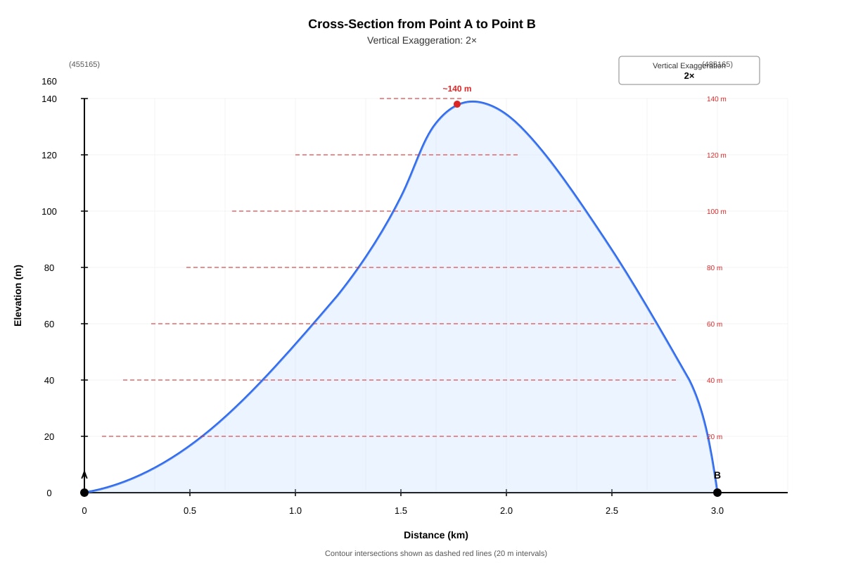
Resource 2: A cross-section diagram showing the profile of the land from point A (grid ref. 455165) to point B (grid ref. 485165), drawn with a vertical exaggeration of 2×.

<image_placeholder> id: Q1-fig1 type: map linked_question: Q1 description: Topographic map extract at 1:50,000 scale showing a coastal region with contour lines at 20 m intervals, a river flowing southeast, a coastal settlement, road networks, and a hill with spot height 142 m. Grid squares from 4512 to 4918. labels: Contour lines (20 m interval), river, coastal settlement, roads, spot height 142 m, grid references, scale bar (1:50,000), north arrow, key/legend values: Spot height: 142 m at grid ref 463178; coastal settlement at 475162; river from 4512 to 4815 must_show: Clear contour spacing, grid lines, settlement symbols, river course, road network, spot height marker, north arrow, scale bar </image_placeholder>

<image_placeholder> id: Q1-fig2 type: diagram linked_question: Q1 description: Cross-section from point A (455165) to point B (485165) showing land profile with vertical exaggeration of 2×. Horizontal axis shows distance in km (0 to 3 km). Vertical axis shows elevation from 0 to 160 m. Profile rises from sea level at A to approximately 140 m near the middle, then descends toward B. labels: Point A, Point B, horizontal axis (distance in km), vertical axis (elevation in m), vertical exaggeration 2×, contour intersections values: Horizontal distance: 3 km; maximum elevation approximately 140 m; vertical exaggeration: 2× must_show: Both axes labelled with units, points A and B marked, profile curve showing hill shape, vertical exaggeration noted </image_placeholder>

1. State the six-figure grid reference of the coastal settlement shown on the map.

[1 mark]

2. What is the straight-line distance, in kilometres, between the coastal settlement at grid reference 475162 and the hill summit at grid reference 463178? Show your working.

[2 marks]

3. Describe the relief of the area between grid squares 4514 and 4814 as shown on the map.

[2 marks]

4. Using evidence from Resource 1, describe the pattern of settlement in the mapped area.

[2 marks]

5. Using Resource 2, calculate the average gradient of the slope from point A to the highest point of the cross-section. Show your working clearly.

[3 marks]

6. State the bearing of the hill summit (463178) from the coastal settlement (475162).

[1 mark]

7. Using both resources, explain why the coastal settlement at 475162 is located where it is.

[3 marks]

8. A student claims that the area between grid squares 4616 and 4816 would be suitable for large-scale agriculture. Using evidence from Resource 1, evaluate this statement.

[3 marks]

Section B: Graph and Data Interpretation (Questions 9–15)

Study the resources below and answer Questions 9–15.

Resource 3: A compound bar graph showing the percentage contribution of different energy sources to total electricity generation in Country X for the years 2000, 2010, and 2020. Energy sources include coal, natural gas, hydroelectric, solar, wind, and nuclear.

<image_placeholder> id: Q9-fig3 type: chart linked_question: Q9 description: Compound (stacked) bar graph showing percentage contribution of six energy sources to total electricity generation in Country X for three years: 2000, 2010, and 2020. Each bar totals 100%. Coal decreases from ~55% (2000) to ~20% (2020). Natural gas increases from ~20% to ~35%. Hydroelectric stable at ~10%. Solar increases from ~0% to ~15%. Wind increases from ~2% to ~12%. Nuclear stable at ~8%. labels: X-axis: Year (2000, 2010, 2020); Y-axis: Percentage of total electricity generation (0–100%); legend showing coal, natural gas, hydroelectric, solar, wind, nuclear with distinct colours/patterns values: 2000: Coal ~55%, Natural gas ~20%, Hydro ~10%, Solar ~0%, Wind ~2%, Nuclear ~8% (remaining ~5% other); 2010: Coal ~40%, Natural gas ~25%, Hydro ~10%, Solar ~8%, Wind ~7%, Nuclear ~8%; 2020: Coal ~20%, Natural gas ~35%, Hydro ~10%, Solar ~15%, Wind ~12%, Nuclear ~8% must_show: Three stacked bars each totalling 100%, clear legend, percentage labels or readable segments, axis labels, title </image_placeholder>

Resource 4: A table showing annual carbon dioxide emissions (in million tonnes) for Country X from 2000 to 2020 at 5-year intervals.

Year	CO₂ Emissions (million tonnes)
2000	450
2005	480
2010	465
2015	420
2020	380

9. According to Resource 3, which energy source contributed the highest percentage to electricity generation in 2000?

[1 mark]

10. Calculate the percentage change in the contribution of coal to electricity generation in Country X between 2000 and 2020. Show your working.

[2 marks]

11. Describe the trend in CO₂ emissions in Country X between 2000 and 2020 as shown in Resource 4.

[2 marks]

12. Using Resources 3 and 4, suggest two reasons why CO₂ emissions in Country X decreased between 2010 and 2020.

[3 marks]

13. A student states: "The increase in solar and wind energy is the only reason CO₂ emissions fell after 2010." Using evidence from both resources, evaluate this statement.

[4 marks]

14. Using Resource 3, identify the energy source that showed the greatest percentage point increase between 2000 and 2020. Calculate this increase.

[2 marks]

15. Based on the data in Resources 3 and 4, describe the relationship between the share of renewable energy and CO₂ emissions in Country X from 2000 to 2020.

[2 marks]

Section C: Statistical and Data Skills (Questions 16–20)

Study the resources below and answer Questions 16–20.

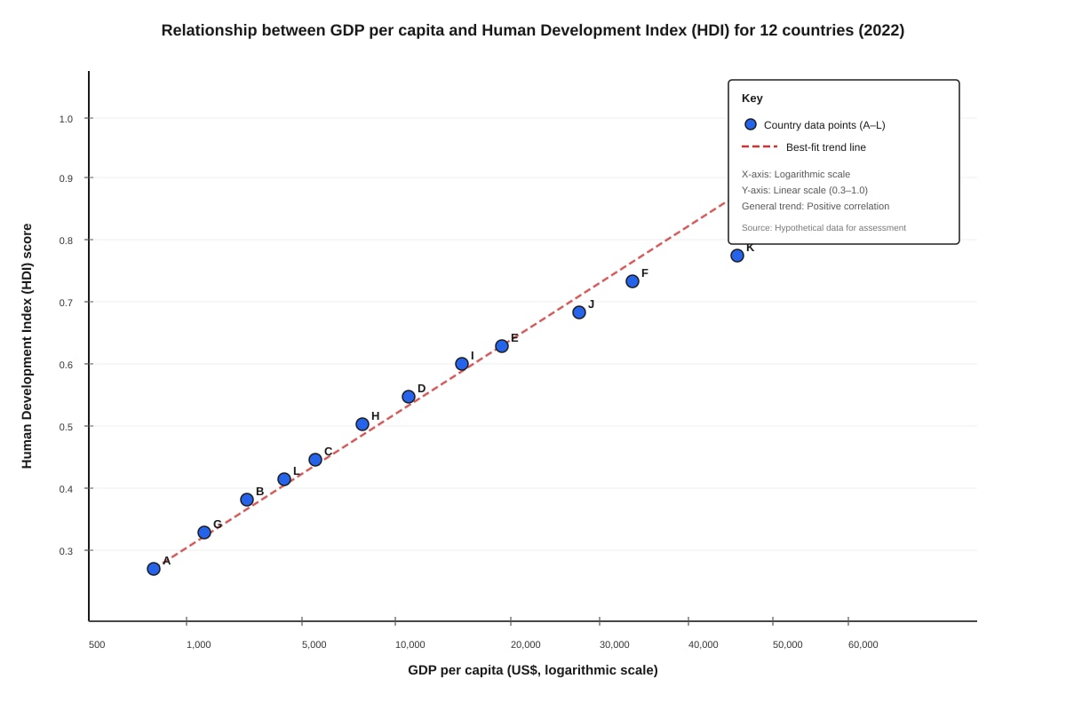
Resource 5: A scatter graph showing the relationship between GDP per capita (in US$) and the Human Development Index (HDI) score for 12 countries in 2022.

<image_placeholder> id: Q16-fig4 type: graph linked_question: Q16 description: Scatter graph plotting GDP per capita (US $, x-axis, logarithmic scale from$ 500 to $60,000) against HDI score (y-axis, 0.3 to 1.0) for 12 countries. General positive correlation visible. Country A: GDP$ 800, HDI 0.42. Country B: GDP $2,500, HDI 0.55. Country C: GDP$ 5,000, HDI 0.62. Country D: GDP $12,000, HDI 0.74. Country E: GDP$ 25,000, HDI 0.82. Country F: GDP $48,000, HDI 0.93. Country G: GDP$ 1,200, HDI 0.48. Country H: GDP $8,000, HDI 0.68. Country I: GDP$ 18,000, HDI 0.79. Country J: GDP $35,000, HDI 0.88. Country K: GDP$ 55,000, HDI 0.95. Country L: GDP $3,500, HDI 0.58. labels: X-axis: GDP per capita (US$ , logarithmic scale); Y-axis: Human Development Index (HDI) score; 12 data points labelled A through L; best-fit line showing positive correlation values: Country A: ( $800, 0.42); Country B: ($ 2,500, 0.55); Country C: ( $5,000, 0.62); Country D: ($ 12,000, 0.74); Country E: ( $25,000, 0.82); Country F: ($ 48,000, 0.93); Country G: ( $1,200, 0.48); Country H: ($ 8,000, 0.68); Country I: ( $18,000, 0.79); Country J: ($ 35,000, 0.88); Country K: ( $55,000, 0.95); Country L: ($ 3,500, 0.58) must_show: Both axes labelled with units, all 12 points labelled A–L, best-fit trend line, title, scale markings </image_placeholder>

Resource 6: A table showing the mean, median, and range of annual rainfall (in mm) for five weather stations in a region.

Weather Station	Mean Annual Rainfall (mm)	Median Annual Rainfall (mm)	Range (mm)
Station P	2,400	2,350	1,800
Station Q	1,800	1,820	950
Station R	3,100	2,900	2,400
Station S	1,200	1,250	600
Station T	2,600	2,580	1,500

16. Using Resource 5, describe the relationship between GDP per capita and HDI score.

[2 marks]

17. Using Resource 5, identify the country that is the outlier and explain why it may not fit the general pattern.

[2 marks]

18. Using Resource 6, calculate the mean of the mean annual rainfall values across all five weather stations. Show your working.

[2 marks]

19. Using Resource 6, compare the rainfall variability at Station P and Station Q. Which station shows more consistent rainfall, and how can you tell?

[2 marks]

20. A geographer wants to present the data from Resource 6 to show both the central tendency and spread of rainfall for each station. Recommend the most appropriate graphical technique and explain why it is suitable.

[3 marks]

End of Quiz

Answers

A-Level Geography H1 Quiz - Map Graph Data Skills

Answer Key

Section A: Map Interpretation (Questions 1–8)

1. State the six-figure grid reference of the coastal settlement shown on the map.

Answer: 475162
[1 mark]

Teaching note: A six-figure grid reference is read as three digits easting (horizontal) followed by three digits northing (vertical). The first two figures of each come from the grid line, and the third is the estimated tenths into the grid square. The question directly gives this in the resource description.

2. What is the straight-line distance, in kilometres, between the coastal settlement at grid reference 475162 and the hill summit at grid reference 463178? Show your working.

Answer:

Easting difference: 475 − 463 = 12 (i.e., 1.2 km on a 1:50,000 map where each grid square = 1 km)
Northing difference: 178 − 162 = 16 (i.e., 1.6 km)
Using Pythagoras' theorem:
$\text{Distance} = \sqrt{(1.2)^2 + (1.6)^2} = \sqrt{1.44 + 2.56} = \sqrt{4.0} = 2.0 \text{ km}$

Answer: 2.0 km
[2 marks] — 1 mark for correct method, 1 mark for correct answer.

Teaching note: On a 1:50,000 map, each grid square represents 1 km × 1 km. The six-figure reference gives coordinates to the nearest 100 m. Students should use the last digit of each three-figure component to estimate the position within the grid square. Pythagoras' theorem is used because the two points are not aligned along a single grid line.

Common mistake: Forgetting to convert grid units to kilometres, or adding the differences instead of using Pythagoras.

3. Describe the relief of the area between grid squares 4514 and 4814 as shown on the map.

Answer:
The area shows varied relief. The land rises from the coast (near sea level) towards the interior, reaching a hill with a spot height of 142 m at grid reference 463178. Contour lines are closely spaced on the western side of the hill, indicating steep slopes, while they are more widely spaced towards the east, indicating gentler gradients. A river flows through the area from grid square 4512 towards 4815, suggesting a valley with lower elevation.

[2 marks] — 1 mark for identifying the general relief (hill/rising land), 1 mark for describing variation (steep vs. gentle slopes, river valley).

Teaching note: "Relief" refers to the shape and elevation of the land surface. Students should use evidence from contour spacing (close = steep, wide = gentle) and spot heights. Always reference specific grid locations for full credit.

4. Using evidence from Resource 1, describe the pattern of settlement in the mapped area.

Answer:
Settlements are concentrated along the coast and near the river. The main coastal settlement is located at grid reference 475162, close to the river mouth. There is also evidence of linear settlement along the road network. Settlements appear to avoid the steep hill area (around 463178), suggesting that rugged terrain discourages habitation.

[2 marks] — 1 mark for identifying coastal/riverine concentration, 1 mark for noting avoidance of steep terrain or linear pattern along roads.

Teaching note: Settlement pattern description should go beyond listing locations. Students should identify the spatial arrangement (clustered, linear, dispersed) and reference specific map evidence (grid references, proximity to features).

5. Using Resource 2, calculate the average gradient of the slope from point A to the highest point of the cross-section. Show your working clearly.

Answer:

Vertical rise from A to highest point: approximately 140 m (from 0 m at A to ~140 m at the peak)
Horizontal distance from A to the highest point: approximately 1.5 km = 1,500 m
Gradient = vertical rise / horizontal distance
$\text{Gradient} = \frac{140}{1500} = 0.0933$
Expressed as a ratio 1 : x:
$x = \frac{1500}{140} = 10.7$
Gradient ≈ 1 : 10.7 (or approximately 1 : 11)

[3 marks] — 1 mark for identifying correct vertical rise, 1 mark for correct horizontal distance, 1 mark for correct calculation and answer.

Teaching note: Gradient is the ratio of vertical change to horizontal distance. Both must be in the same units. The vertical exaggeration (2×) on the cross-section means the visual slope appears steeper than reality — students must use the actual values from the axes, not estimate from the visual steepness.

Common mistake: Using the exaggerated vertical scale to read values, or forgetting to convert km to m.

6. State the bearing of the hill summit (463178) from the coastal settlement (475162).

Answer:

The hill summit is to the west (lower easting: 463 vs 475) and to the north (higher northing: 178 vs 162) of the coastal settlement.
This places it in the north-west direction.
More precisely, the angle west of north:
$\tan \theta = \frac{\text{easting difference}}{\text{northing difference}} = \frac{12}{16} = 0.75$
$\theta = \tan^{-1}(0.75) \approx 36.9°$
Bearing = 360° − 36.9° = 323° (or approximately 323°)

Answer: Approximately 323° (or NW)
[1 mark]

Teaching note: Bearings are measured clockwise from north (0°/360°). Students should draw a north line at the starting point, then measure the clockwise angle to the destination. A rough directional answer (NW) may receive credit at H1 level, but a precise bearing demonstrates stronger skills.

7. Using both resources, explain why the coastal settlement at 475162 is located where it is.

Answer:
The coastal settlement is located at 475162 due to several favourable site factors:

Access to water and trade: Its coastal position provides access to the sea for fishing, trade, and transport. The proximity to the river mouth (the river flows to 4815, near the settlement) also provides freshwater and a sheltered harbour.
Flat land for construction: Resource 2 shows that the coastal area near point A is at or near sea level with gentle gradients, making it suitable for building infrastructure and housing.
Transport links: The settlement is connected by road networks (visible on Resource 1), facilitating movement of goods and people.
Avoidance of steep terrain: The settlement is located away from the steep hill slopes (around 463178), where construction would be difficult and costly.

[3 marks] — 1 mark for each valid point with evidence from the resources, up to 3 marks.

Teaching note: Settlement site factors include water supply, flat land, transport access, defence, and resources. Students must link each reason to specific evidence from the resources (grid references, contour patterns, cross-section data) for full marks.

8. A student claims that the area between grid squares 4616 and 4816 would be suitable for large-scale agriculture. Using evidence from Resource 1, evaluate this statement.

Answer:
Supporting the claim:

The area appears to have relatively flat or gently sloping land (contour lines are likely more widely spaced in this zone), which is suitable for mechanised farming.
The proximity to the river provides a reliable water source for irrigation.
The road network provides access for transporting agricultural produce.

Challenging the claim:

If the area is near the river, it may be prone to flooding, which could damage crops.
The area may already be occupied by the coastal settlement or other land uses (e.g., residential, commercial), limiting available farmland.
If contour lines are close together in parts of this area, the terrain may be too steep for large-scale farming.

Conclusion: The suitability depends on the specific terrain and existing land use. While flat land and water access are positive factors, flood risk and competing land uses may limit agricultural potential.

[3 marks] — 1 mark for evidence supporting suitability, 1 mark for evidence challenging suitability, 1 mark for a reasoned conclusion.

Teaching note: Evaluation questions require students to consider both sides and reach a supported judgement. "Evaluate" does not mean simply agreeing or disagreeing — students must weigh evidence and qualify their conclusion.

Section B: Graph and Data Interpretation (Questions 9–15)

9. According to Resource 3, which energy source contributed the highest percentage to electricity generation in 2000?

Answer: Coal (~55%)
[1 mark]

Teaching note: Students should read the stacked bar for 2000 and identify the largest segment. Coal is clearly the dominant source at approximately 55%.

10. Calculate the percentage change in the contribution of coal to electricity generation in Country X between 2000 and 2020. Show your working.

Answer:

Coal contribution in 2000: ~55%
Coal contribution in 2020: ~20%
Change = 20% − 55% = −35 percentage points
Percentage change = (change / original) × 100
$\text{Percentage change} = \frac{-35}{55} \times 100 = -63.6\%$

Answer: Approximately −63.6% (a decrease of 63.6%)
[2 marks] — 1 mark for correct method, 1 mark for correct answer.

Teaching note: Percentage change = ((new − old) / old) × 100. The negative sign indicates a decrease. Students should be careful to distinguish between "percentage point change" (−35 pp) and "percentage change" (−63.6%). The question asks for percentage change.

11. Describe the trend in CO₂ emissions in Country X between 2000 and 2020 as shown in Resource 4.

Answer:
CO₂ emissions in Country X showed an overall decreasing trend between 2000 and 2020, but with fluctuations. Emissions rose from 450 million tonnes in 2000 to a peak of 480 million tonnes in 2005. They then declined to 465 million tonnes in 2010, fell further to 420 million tonnes in 2015, and reached 380 million tonnes in 2020. The overall decrease from 2000 to 2020 was 70 million tonnes (from 450 to 380).

[2 marks] — 1 mark for identifying the overall decreasing trend, 1 mark for describing the fluctuation (rise then fall) with specific data values.

Teaching note: When describing trends, students should: (1) state the overall direction, (2) note any fluctuations or anomalies, and (3) use specific data values to support their description. Avoid vague language like "it went up and down."

12. Using Resources 3 and 4, suggest two reasons why CO₂ emissions in Country X decreased between 2010 and 2020.

Answer:

Shift from coal to natural gas: Resource 3 shows that coal's share of electricity generation fell from ~40% in 2010 to ~20% in 2020, while natural gas increased from ~25% to ~35%. Natural gas produces less CO₂ per unit of energy than coal, so this fuel switch would reduce emissions.
Growth of renewable energy: Solar energy increased from ~8% to ~15% and wind energy from ~7% to ~12% between 2010 and 2020. These renewable sources produce negligible CO₂ during operation, displacing fossil fuel generation and reducing overall emissions.

[3 marks] — 1 mark for each valid reason with supporting data from Resource 3, up to 2 marks, plus 1 mark for linking the energy changes to CO₂ reduction.

Teaching note: Students must use evidence from the resources, not general knowledge. Each reason should reference specific percentage changes from Resource 3 and explain the causal link to CO₂ reduction.

13. A student states: "The increase in solar and wind energy is the only reason CO₂ emissions fell after 2010." Using evidence from both resources, evaluate this statement.

Answer:
Agreeing partially:

Solar and wind energy did increase significantly (solar from ~8% to ~15%, wind from ~7% to ~12%), and these sources produce minimal CO₂, contributing to the emissions decline.

However, other factors were also important:

Coal decline: Coal's share fell from ~40% to ~20%, a 20 percentage point decrease. Since coal is the most carbon-intensive fuel, this reduction would have a substantial impact on CO₂ emissions — arguably larger than the solar/wind increase.
Natural gas increase: Natural gas rose from ~25% to ~35%. While still a fossil fuel, gas produces roughly half the CO₂ of coal per unit of energy, so this substitution also contributed to lower emissions.
Other factors not shown: The data does not account for changes in energy efficiency, industrial output, transport emissions, or population — all of which could influence total CO₂ emissions.

Conclusion: The increase in solar and wind energy contributed to falling CO₂ emissions, but it was not the only reason. The decline in coal use and the shift to natural gas were also significant factors. The statement is therefore an oversimplification.

[4 marks] — 1 mark for acknowledging the role of solar/wind, 1 mark for identifying other factors from the data, 1 mark for explaining why these other factors matter, 1 mark for a reasoned conclusion.

Teaching note: Evaluation of statements requires students to assess the validity of a claim using evidence. The strongest answers acknowledge partial truth while identifying limitations and alternative explanations.

14. Using Resource 3, identify the energy source that showed the greatest percentage point increase between 2000 and 2020. Calculate this increase.

Answer:

Solar: from ~0% to ~15% → increase of ~15 percentage points
Wind: from ~2% to ~12% → increase of ~10 percentage points
Natural gas: from ~20% to ~35% → increase of ~15 percentage points
Hydroelectric: stable at ~10% → no change
Nuclear: stable at ~8% → no change
Coal: decreased

Both solar and natural gas show the greatest percentage point increase of approximately 15 percentage points. However, solar's percentage increase is larger in relative terms (from near zero).

Answer: Solar energy (and natural gas), with an increase of approximately 15 percentage points.
[2 marks] — 1 mark for correct identification, 1 mark for correct calculation.

Teaching note: "Percentage point increase" is the arithmetic difference between two percentages, not the percentage change. Students should calculate the difference for each source and compare.

15. Based on the data in Resources 3 and 4, describe the relationship between the share of renewable energy and CO₂ emissions in Country X from 2000 to 2020.

Answer:
As the share of renewable energy (solar + wind + hydroelectric) increased from approximately 12% in 2000 (0% + 2% + 10%) to approximately 37% in 2020 (15% + 12% + 10%), CO₂ emissions decreased from 450 million tonnes to 380 million tonnes. This shows an inverse (negative) relationship: as renewable energy's contribution to electricity generation grew, CO₂ emissions fell. The most significant decline in emissions occurred after 2010, coinciding with the period of most rapid growth in solar and wind energy.

[2 marks] — 1 mark for identifying the inverse relationship, 1 mark for supporting with specific data values from both resources.

Teaching note: When describing relationships between two variables, students should: (1) state the type of relationship (positive, inverse, or no clear relationship), (2) describe how both variables changed over time, and (3) use specific data to support the description.

Section C: Statistical and Data Skills (Questions 16–20)

16. Using Resource 5, describe the relationship between GDP per capita and HDI score.

Answer:
There is a positive correlation between GDP per capita and HDI score. As GDP per capita increases, the HDI score also tends to increase. Countries with low GDP per capita (e.g., Country A at $800, HDI 0.42) have low HDI scores, while countries with high GDP per capita (e.g., Country K at$ 55,000, HDI 0.95) have high HDI scores. However, the relationship is not perfectly linear — the rate of HDI increase slows at higher income levels, suggesting diminishing returns.

[2 marks] — 1 mark for identifying the positive correlation, 1 mark for describing the pattern with reference to specific data points.

Teaching note: A positive correlation means both variables increase together. Students should reference specific countries and values from the scatter graph. Noting the non-linear nature (diminishing returns) demonstrates higher-level analysis.

17. Using Resource 5, identify the country that is the outlier and explain why it may not fit the general pattern.

Answer:
Country G (GDP $1,200, HDI 0.48) appears to be a potential outlier. It has a higher GDP per capita than Country A ($ 800) but its HDI score (0.48) is only slightly higher than Country A's (0.42), despite the $400 difference in GDP. Alternatively, Country G's HDI is lower than expected for its income level when compared to the general trend line — Country B has a similar HDI (0.55) but at$ 2,500 GDP, suggesting Country G underperforms relative to the trend.

Country G may not fit the pattern due to factors such as political instability, unequal income distribution, poor governance, conflict, or limited investment in health and education — factors that prevent economic wealth from translating into human development.

[2 marks] — 1 mark for correctly identifying the outlier with data, 1 mark for a plausible explanation.

Teaching note: An outlier is a data point that deviates significantly from the general trend. Students should compare the outlier to the best-fit line or to countries with similar GDP/HDI values. Explanations should reference real-world factors that affect HDI independently of GDP.

18. Using Resource 6, calculate the mean of the mean annual rainfall values across all five weather stations. Show your working.

Answer:
$\text{Mean} = \frac{2400 + 1800 + 3100 + 1200 + 2600}{5} = \frac{11100}{5} = 2220 \text{ mm}$

Answer: 2,220 mm
[2 marks] — 1 mark for correct method (summing and dividing by 5), 1 mark for correct answer.

Teaching note: The mean is calculated by summing all values and dividing by the number of values. Students should show their working to receive full marks even if the final answer has a minor arithmetic error.

19. Using Resource 6, compare the rainfall variability at Station P and Station Q. Which station shows more consistent rainfall, and how can you tell?

Answer:
Station Q shows more consistent rainfall than Station P. This is evidenced by:

Range: Station Q has a range of 950 mm, while Station P has a range of 1,800 mm. A smaller range indicates less variability.
Mean vs. Median: At Station Q, the mean (1,800 mm) and median (1,820 mm) are very close, suggesting a symmetrical distribution with few extreme values. At Station P, the mean (2,400 mm) and median (2,350 mm) differ more, and the larger range suggests greater spread.

Answer: Station Q shows more consistent rainfall, as indicated by its smaller range (950 mm vs. 1,800 mm).
[2 marks] — 1 mark for identifying Station Q as more consistent, 1 mark for using range (and optionally mean-median comparison) as evidence.

Teaching note: Variability can be assessed using range, standard deviation, or by comparing mean and median. A smaller range and closer mean-median values both indicate more consistent (less variable) data.

Answer:
The most appropriate technique is a box-and-whisker plot (box plot).

Why it is suitable:

A box plot displays the median (central tendency), interquartile range (spread of the middle 50% of data), and the full range (minimum to maximum values) for each station.
It allows easy comparison of both central tendency and variability across all five stations on a single graph.
Outliers can be identified if present.
It is more informative than a simple bar chart (which only shows mean) because it reveals the distribution shape and spread.

Alternative: A bar chart with error bars could also be used, where bars represent the mean and error bars show the range or standard deviation. However, this is less informative than a box plot because it does not show the median or quartiles.

[3 marks] — 1 mark for recommending box-and-whisker plot, 1 mark for explaining how it shows central tendency, 1 mark for explaining how it shows spread and enables comparison.

Teaching note: Students should be familiar with multiple graphical techniques and be able to justify their choice based on the data characteristics and the purpose of the presentation. Box plots are ideal for comparing distributions across categories.

End of Answer Key

Mark Summary

Section	Questions	Marks
A: Map Interpretation	1–8	17
B: Graph and Data Interpretation	9–15	16
C: Statistical and Data Skills	16–20	11
Total	20 questions	44

Note: The total marks for this quiz are 44, distributed across 20 questions. This is appropriate for a 60-minute quiz at A-Level H1 Geography, allowing approximately 1.4 minutes per mark.