AI Generated Quiz
A Level H2 Economics Microeconomics Quiz
Free A Level H2 Econs Microeconomics quiz, LongCat AI version, with questions, answers, and A Level-style practice for Singapore students.
These static practice materials are generated from the site's syllabus and paper-generation workflow, with source and model context shown so students and parents can evaluate the material before use.
Questions
A-Level Economics H2 Quiz - Microeconomics
Name: ________________________ Class: ________________________ Date: ________________________ Score: ______ / 60
Duration: 75 minutes Total Marks: 60
Instructions
- Answer all questions in the spaces provided.
- Read each question carefully before writing your response.
- For calculation questions, show all working clearly.
- For essay-style questions, use relevant economic terminology, diagrams where appropriate, and real-world examples to support your analysis.
- Quality of written communication will be assessed in extended responses.
Section A: Central Economic Problem & Price Mechanism (Questions 1–5)
Answer all questions. Each question is worth 2 marks. Total: 10 marks.
1. A small island nation has 200 units of labour and 100 units of capital. It can produce either rice or fish. The production possibilities are shown below:
| Combination | Rice (tonnes) | Fish (tonnes) |
|---|---|---|
| A | 0 | 500 |
| B | 200 | 450 |
| C | 400 | 350 |
| D | 600 | 200 |
| E | 800 | 0 |
(a) What is the opportunity cost of increasing rice production from 200 tonnes to 400 tonnes?
(b) Explain whether the opportunity cost of rice is constant or increasing as more rice is produced. Justify your answer using the data above.
2. The cross-price elasticity of demand between Good X and Good Y is measured at +2.5. The price of Good Y increases by 8%.
(a) State the relationship between Good X and Good Y.
(b) Calculate the percentage change in quantity demanded of Good X. Show your working.
3. A firm sells a luxury handbag. When the price was 800,monthlysaleswere1,200units.Afterapriceincreaseto1,000, monthly sales fell to 800 units.
(a) Calculate the price elasticity of demand using the midpoint (arc elasticity) method. Show your working.
(b) Based on your calculation, state whether demand is elastic, inelastic, or unitary elastic. Explain what this means for the firm's total revenue after the price increase.
4. Explain two factors that would cause the supply curve for electric vehicles to shift to the right.
Factor 1: _______________________________________________________________
Factor 2: _______________________________________________________________
5. Using a demand and supply diagram, explain how a government-imposed price ceiling set below the equilibrium price creates a shortage in the market. In your answer, refer to the diagram below.
Image pending generation: graph for Q5.
Section B: Market Structures (Questions 6–10)
Answer all questions. Total: 20 marks.
6. (4 marks)
The table below shows the cost and revenue data for a firm operating in a perfectly competitive market.
| Output (units) | Total Cost ($) | Total Revenue ($) | Marginal Cost ($) | Marginal Revenue ($) |
|---|---|---|---|---|
| 0 | 50 | 0 | — | — |
| 1 | 70 | 30 | 20 | 30 |
| 2 | 85 | 60 | 15 | 30 |
| 3 | 105 | 90 | 20 | 30 |
| 4 | 130 | 120 | 25 | 30 |
| 5 | 160 | 150 | 30 | 30 |
| 6 | 195 | 180 | 35 | 30 |
| 7 | 235 | 210 | 40 | 30 |
(a) At what output level does the firm maximise profit? Explain your reasoning.
(b) Calculate the firm's maximum profit. Show your working.
7. (4 marks)
Image pending generation: graph for Q7.
Using the diagram above:
(a) Identify the profit-maximising price and quantity for the monopoly.
(b) Shade and label the area representing supernormal profit on the diagram. Calculate the value of this profit.
(c) Explain why a monopoly can sustain supernormal profit in the long run, whereas a firm in perfect competition cannot.
8. (4 marks)
Compare and contrast the characteristics of an oligopoly and monopolistic competition. In your answer, refer to at least three distinguishing features and provide a real-world example of each market structure.
9. (4 marks)
A dominant firm in Singapore's telecommunications market is considering whether to engage in price leadership. Explain the concept of price leadership and discuss one advantage and one disadvantage of this strategy for the firm.
10. (4 marks)
Explain the concept of allocative efficiency. Under which market structure(s) is allocative efficiency achieved in the long run? Justify your answer with reference to the relationship between price and marginal cost.
Section C: Market Failure & Government Intervention (Questions 11–15)
Answer all questions. Total: 15 marks.
11. (3 marks)
The production of cement generates negative externalities in the form of air pollution. The marginal external cost (MEC) is estimated at $15 per tonne of cement produced.
(a) Explain what is meant by a negative externality and why it leads to market failure.
(b) On the diagram below, indicate the socially optimal level of output and explain how it differs from the free market equilibrium.
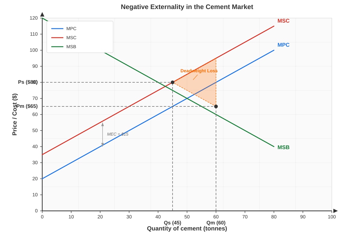
Generated graph for Q11.
12. (3 marks)
(a) Define a public good and explain the two key characteristics that distinguish it from a private good.
(b) Explain why the free market would under-provide public goods. Use the concept of the free-rider problem in your answer.
13. (3 marks)
The Singapore government provides subsidies for SkillsFuture courses to encourage lifelong learning.
(a) Explain why SkillsFuture courses may be considered a merit good.
(b) Discuss whether a subsidy is the most effective government intervention to increase uptake of SkillsFuture courses. Consider one alternative policy.
14. (3 marks)
Explain how asymmetric information in the market for second-hand cars (the "lemons problem") leads to market failure. In your answer, explain how this problem might be reduced.
15. (3 marks)
A government is considering two policies to reduce carbon emissions from the transport sector: (i) a carbon tax on petrol, or (ii) tradable pollution permits for transport companies.
Compare the effectiveness of these two policies in achieving the socially optimal level of emissions. In your answer, consider efficiency, certainty of outcome, and administrative feasibility.
Section D: Extended Response (Questions 16–20)
Answer all questions. Total: 15 marks.
16. (5 marks)
The demand and supply schedules for the market for organic vegetables in Singapore are given below:
| Price ($/kg) | Quantity Demanded (kg per week) | Quantity Supplied (kg per week) |
|---|---|---|
| 4 | 8,000 | 2,000 |
| 6 | 6,000 | 4,000 |
| 8 | 4,000 | 6,000 |
| 10 | 2,000 | 8,000 |
| 12 | 1,000 | 10,000 |
(a) Determine the equilibrium price and quantity. Show how you know this is the equilibrium.
(b) The government imposes a specific tax of $3 per kg on organic vegetable producers. Calculate the new equilibrium price paid by consumers and the new equilibrium quantity. Show your working.
(c) Calculate the total tax revenue collected by the government.
(d) Calculate the incidence of the tax on consumers and producers respectively.
17. (5 marks)
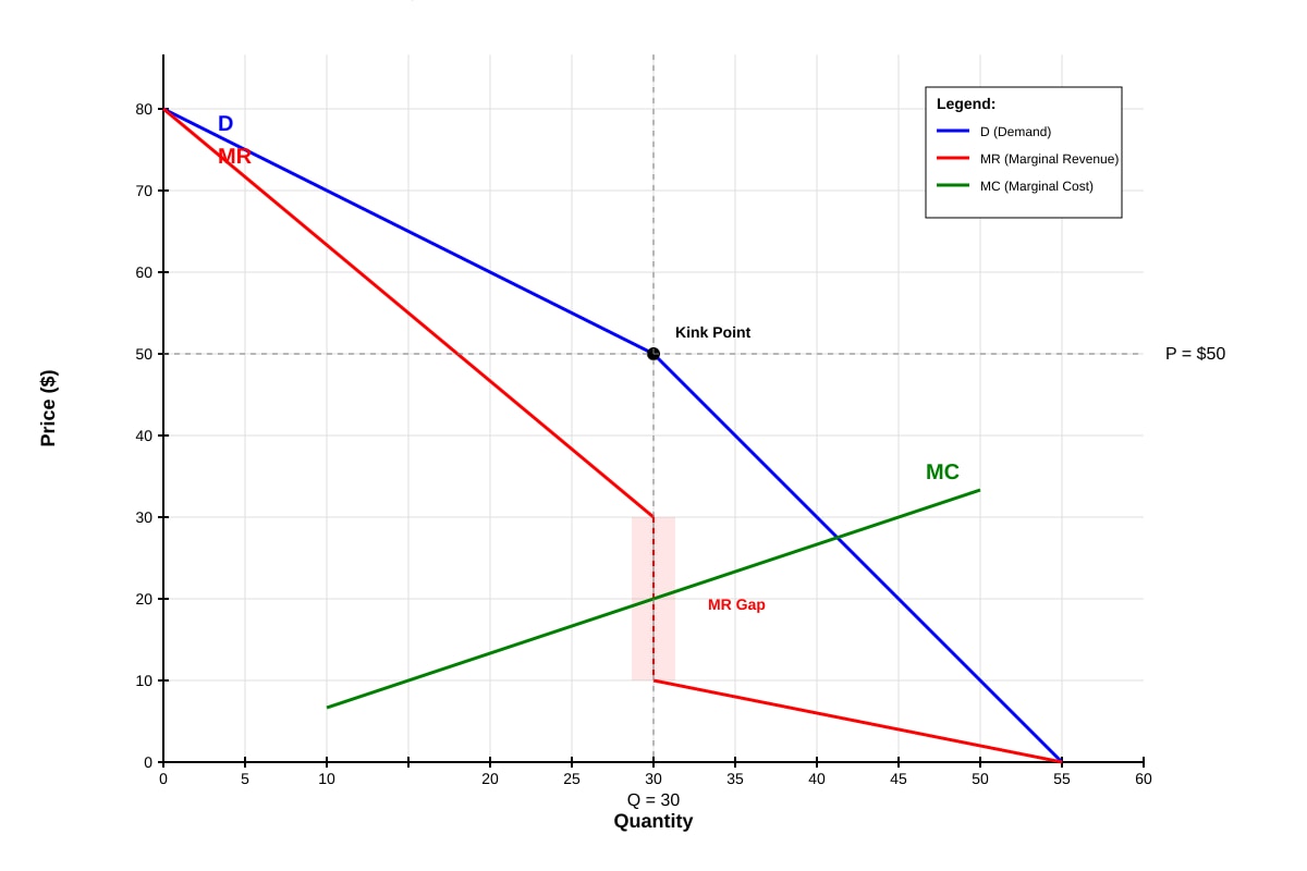
Generated graph for Q17.
Using the kinked demand curve diagram above:
(a) Explain why the demand curve is kinked at the prevailing price of $50.
(b) Explain why the marginal revenue curve has a vertical discontinuity at the prevailing quantity of 30 units.
(c) Using the diagram, explain why oligopolists tend to maintain stable prices even when their costs change.
18. (5 marks)
"Government intervention in markets always leads to a more efficient outcome than the free market."
Discuss this statement with reference to at least two forms of government intervention and two examples of market failure. In your answer, consider both the potential benefits and limitations of government action.
19. (5 marks)
A pharmaceutical company holds a patent on a life-saving drug, giving it monopoly power in the market. The firm currently charges 500perdose,andthemarginalcostofproductionis50 per dose.
(a) Using a diagram, explain how the monopoly pricing of this drug leads to allocative inefficiency.
(b) Discuss whether the government should regulate the price of this drug. In your answer, consider the trade-off between consumer welfare and the incentive for innovation.
20. (5 marks)
Singapore's hawker centres provide affordable food to the population. The government subsidises stall rentals and provides direct provision of hawker centre infrastructure.
(a) Explain why the government might consider hawker food to have characteristics of a merit good.
(b) Evaluate the effectiveness of government subsidies and direct provision as methods of ensuring affordable hawker food in Singapore. In your answer, consider alternative policies and potential unintended consequences.
Answers
A-Level Economics H2 Quiz - Microeconomics
Answer Key & Marking Scheme
Total Marks: 60
Section A: Central Economic Problem & Price Mechanism (Questions 1–5)
Question 1 (2 marks)
(a) Opportunity cost of increasing rice from 200 to 400 tonnes (1 mark)
When rice production increases from 200 to 400 tonnes (moving from Combination B to C), fish production falls from 450 to 350 tonnes.
Opportunity cost = 450 − 350 = 100 tonnes of fish
Mark: 1 mark for correct answer of 100 tonnes of fish.
(b) Whether opportunity cost is constant or increasing (1 mark)
The opportunity cost is increasing. Justification using the data:
- From A to B: 200 tonnes of rice costs 50 fish → 1 rice = 0.25 fish
- From B to C: 200 tonnes of rice costs 100 fish → 1 rice = 0.5 fish
- From C to D: 200 tonnes of rice costs 150 fish → 1 rice = 0.75 fish
- From D to E: 200 tonnes of rice costs 200 fish → 1 rice = 1 fish
The opportunity cost per unit of rice increases as more rice is produced, indicating an increasing opportunity cost (the PPC is concave/bowed outward). This reflects the fact that resources are not equally suited to the production of both goods.
Mark: 1 mark for identifying increasing opportunity cost with correct justification from the data.
Question 2 (2 marks)
(a) Relationship between Good X and Good Y (1 mark)
The cross-price elasticity of demand is positive (+2.5), which means Good X and Good Y are substitutes. When the price of Good Y rises, consumers switch to Good X, increasing the quantity demanded of Good X.
Mark: 1 mark for identifying substitutes.
(b) Percentage change in quantity demanded of Good X (1 mark)
Formula: EXY=%ΔPY%ΔQX
Rearranging: %ΔQX=EXY×%ΔPY=2.5×8%=+20%
The quantity demanded of Good X increases by 20%.
Mark: 1 mark for correct calculation (+20%).
Question 3 (2 marks)
(a) Price elasticity of demand using midpoint method (1 mark)
Midpoint formula: Ed=ΔP/PavgΔQ/Qavg
- ΔQ=800−1200=−400
- Qavg=(1200+800)/2=1000
- ΔP=1000−800=200
- Pavg=(800+1000)/2=900
Ed=200/900−400/1000=0.222−0.4=-1.8
(Or expressed as |1.8| in absolute terms.)
Mark: 1 mark for correct calculation showing working.
(b) Elasticity classification and revenue impact (1 mark)
Since |E_d| = 1.8 > 1, demand is elastic. This means the percentage change in quantity demanded is greater than the percentage change in price. When demand is elastic, a price increase leads to a decrease in total revenue (because the loss in revenue from selling fewer units outweighs the gain from the higher price).
Mark: 1 mark for identifying elastic demand and correctly explaining the revenue impact.
Question 4 (2 marks)
Two factors causing the supply curve for electric vehicles to shift right (1 mark each):
Factor 1: A decrease in the cost of production inputs, such as a fall in the price of lithium batteries or other raw materials. Lower production costs mean firms are willing to supply more at each price level.
Factor 2: Technological advancement that improves the efficiency of EV manufacturing. Better technology reduces the cost per unit and increases the quantity that can be produced at any given price.
(Other acceptable answers: government subsidies to EV producers, entry of new firms into the market, decrease in taxes on EV production, favourable expectations about future prices.)
Mark: 1 mark per valid factor, up to 2 marks.
Question 5 (2 marks)
Explanation of how a price ceiling creates shortage (2 marks):
A price ceiling is a maximum legal price set by the government. When set below the equilibrium price (1200<2000), it creates a shortage because:
- At the ceiling price of $1200, the quantity demanded (800 units) exceeds the quantity supplied (300 units).
- The shortage = 800 − 300 = 500 units.
- This occurs because the artificially low price encourages more consumers to demand rental housing (movement along the demand curve) while discouraging landlords from supplying rental units (movement along the supply curve).
- The result is excess demand that cannot be resolved through price adjustment since the price cannot rise to clear the market.
Mark: 1 mark for identifying that Qd > Qs at the ceiling price. 1 mark for explaining the mechanism (price too low, quantity demanded increases, quantity supplied decreases, resulting in shortage).
Section B: Market Structures (Questions 6–10)
Question 6 (4 marks)
(a) Profit-maximising output level (2 marks)
The firm maximises profit where Marginal Revenue (MR) = Marginal Cost (MC).
From the table, MR = MC = $30 at output = 5 units.
At output 4: MC (25)<MR(30) → firm should increase output. At output 5: MC (30)=MR(30) → profit maximised. At output 6: MC (35)>MR(30) → firm should decrease output.
Profit-maximising output = 5 units.
Mark: 1 mark for identifying MR = MC condition. 1 mark for correct output of 5 units with justification.
(b) Maximum profit calculation (2 marks)
At output = 5:
- Total Revenue = $150
- Total Cost = $160
- Profit = TR − TC = 150−160 = −$10 (a loss)
The firm makes a **loss of 10∗∗attheprofit−maximisingoutput.However,sincethequestionasksformaximumprofit,theansweris−10 (or a loss of $10). The firm is making losses but this is the best it can do in the short run if price exceeds average variable cost.
Mark: 1 mark for correct TR and TC values at Q=5. 1 mark for correct profit calculation (−$10).
Question 7 (4 marks)
(a) Profit-maximising price and quantity (1 mark)
From the diagram, the profit-maximising output is where MR = MC, which occurs at Qm = 20 units. The corresponding price on the demand curve is Pm = $60.
Mark: 1 mark for correct identification of Pm = $60 and Qm = 20.
(b) Supernormal profit calculation (1 mark)
Supernormal profit = (Price − Average Cost) × Quantity = (60−40) × 20 = 20×20=∗∗400**
The supernormal profit is the shaded rectangle between Pm (60)andAC(40) over the quantity of 20 units.
Mark: 1 mark for correct calculation ($400).
(c) Why monopoly sustains supernormal profit in the long run (2 marks)
A monopoly can sustain supernormal profit in the long run because of barriers to entry. These barriers (such as patents, control of essential resources, economies of scale, or government licences) prevent new firms from entering the market and competing away the supernormal profit.
In perfect competition, there are no barriers to entry. If firms earn supernormal profit, new firms are attracted to the market, increasing supply, driving down price, and eliminating supernormal profit in the long run. The monopoly's barriers prevent this process.
Mark: 1 mark for identifying barriers to entry. 1 mark for contrasting with perfect competition (free entry eliminates supernormal profit).
Question 8 (4 marks)
Comparison of oligopoly and monopolistic competition (4 marks):
| Feature | Oligopoly | Monopolistic Competition |
|---|---|---|
| Number of firms | Few dominant firms | Many firms |
| Product differentiation | Products may be homogeneous or differentiated | Products are differentiated |
| Barriers to entry | Significant barriers to entry | Low/no barriers to entry |
| Interdependence | Firms are interdependent (consider rivals' reactions) | Firms act independently |
| Long-run profit | Can earn supernormal profit | Zero supernormal profit (normal profit only) |
Real-world examples:
- Oligopoly: Singapore telecommunications market (Singtel, StarHub, M1)
- Monopolistic competition: Restaurants, hairdressers, clothing retailers
Marking:
- 1 mark for each valid distinguishing feature (up to 3 marks for features)
- 1 mark for real-world examples (at least one for each structure)
Question 9 (4 marks)
Price leadership (2 marks):
Price leadership occurs when one dominant firm in an oligopoly sets the price and other firms in the industry follow. The price leader is typically the largest or most efficient firm. Other firms follow because they fear that if they set a higher price, they will lose market share, and if they set a lower price, a price war may erupt that harms all firms.
Advantage (1 mark):
- Price stability: Price leadership avoids destructive price wars, providing certainty for firms in planning and investment. It maintains industry profitability.
Disadvantage (1 mark):
- Reduced competition: Price leadership may lead to prices that are higher than under competitive conditions, reducing consumer welfare. It may also be seen as anti-competitive behaviour.
(Other valid advantages: reduces uncertainty, avoids price wars. Other disadvantages: may be illegal under competition law, smaller firms may be forced to follow even if the price is not optimal for them.)
Mark: 2 marks for explanation of price leadership. 1 mark for advantage. 1 mark for disadvantage.
Question 10 (4 marks)
Allocative efficiency (4 marks):
Allocative efficiency occurs when resources are allocated in a way that maximises total social welfare. It is achieved when Price (P) = Marginal Cost (MC), meaning the value consumers place on the last unit produced (reflected by the price they are willing to pay) equals the cost of producing that unit.
Market structure(s) achieving allocative efficiency in the long run:
-
Perfect competition achieves allocative efficiency in the long run. In long-run equilibrium, firms produce at the minimum point of the long-run average cost curve where P = MC = minimum LRAC. This ensures that the right quantity of goods is produced from society's perspective.
-
Monopoly does NOT achieve allocative efficiency because the monopolist restricts output to raise price above marginal cost (P > MC), resulting in underproduction and deadweight loss.
-
Monopolistic competition does NOT achieve allocative efficiency in the long run because firms produce where P > MC (though the deviation is smaller than in monopoly).
-
Oligopoly generally does NOT achieve allocative efficiency as firms restrict output to maintain prices above marginal cost.
Mark: 2 marks for defining allocative efficiency (P = MC). 2 marks for identifying perfect competition and explaining why, with reference to at least one other market structure for contrast.
Section C: Market Failure & Government Intervention (Questions 11–15)
Question 11 (3 marks)
(a) Negative externality and market failure (1 mark)
A negative externality is a cost imposed on third parties who are not involved in the production or consumption of a good. In the case of cement production, air pollution harms the health of nearby residents and damages the environment.
It leads to market failure because the free market only considers private costs (MPC) and ignores the external costs (MEC). The market equilibrium (where MPC = MSB) results in overproduction (Qm = 60) compared to the socially optimal level (Qs = 45). The difference represents a deadweight loss to society.
Mark: 1 mark for defining negative externality and explaining why it causes market failure (overproduction due to external costs not being accounted for).
(b) Socially optimal output (2 marks)
The socially optimal level of output is where MSC = MSB, which occurs at Qs = 45 tonnes and Ps = $80.
This differs from the free market equilibrium (Qm = 60, Pm = 65)becausethefreemarketignoresthemarginalexternalcostof15 per tonne. The free market overproduces by 15 tonnes (60 − 45), resulting in a deadweight loss equal to the area of the triangle between MSC and MSB from Q = 45 to Q = 60.
Mark: 1 mark for identifying Qs = 45. 1 mark for explaining the difference from free market equilibrium.
Question 12 (3 marks)
(a) Public good definition and characteristics (2 marks)
A public good is a good that is non-excludable and non-rivalrous in consumption.
- Non-excludable: Once the good is provided, it is impossible or very costly to prevent anyone from consuming it, even if they do not pay for it.
- Non-rivalrous: One person's consumption of the good does not reduce the amount available for others to consume.
Examples: national defence, street lighting, public parks.
Mark: 1 mark for definition. 1 mark for explaining both characteristics.
(b) Free-rider problem and under-provision (1 mark)
Because public goods are non-excludable, individuals have an incentive to free-ride — to enjoy the benefits of the good without paying for it. Since everyone has this incentive, private firms cannot charge consumers and therefore will not provide the good profitably. This leads to under-provision (or complete non-provision) of public goods by the free market, resulting in market failure.
Mark: 1 mark for explaining the free-rider problem and linking it to under-provision.
Question 13 (3 marks)
(a) SkillsFuture as a merit good (1 mark)
A merit good is a good that is under-consumed in the free market because individuals underestimate its long-term benefits (information failure) or because it generates positive externalities. SkillsFuture courses may be considered a merit good because:
- Individuals may not fully appreciate the long-term benefits of upskilling (information failure/myopia).
- An upskilled workforce generates positive externalities for the economy (higher productivity, innovation, economic growth).
Mark: 1 mark for explaining why SkillsFuture courses have merit good characteristics.
(b) Subsidy effectiveness and alternative policy (2 marks)
Subsidy: A subsidy reduces the price of SkillsFuture courses, increasing uptake. It is effective because it directly addresses the under-consumption problem by making courses more affordable. However, subsidies are costly to the government and may fund courses that individuals would have taken anyway (deadweight loss of subsidy).
Alternative policy — Regulation/compulsory training: The government could mandate certain training requirements for specific industries. This ensures uptake but may be inflexible and impose costs on firms.
Alternative policy — Information campaigns: Providing better information about the benefits of SkillsFuture courses could address the information failure directly. This is less costly but may be insufficient on its own.
Mark: 1 mark for discussing subsidy effectiveness. 1 mark for considering an alternative policy with reasoning.
Question 14 (3 marks)
Asymmetric information and the lemons problem (3 marks):
In the second-hand car market, sellers have more information about the quality of the car than buyers. This asymmetric information leads to the "lemons problem" (Akerlof, 1970):
- Buyers cannot distinguish between high-quality cars ("peaches") and low-quality cars ("lemons").
- Buyers are only willing to pay an average price that reflects the expected quality.
- Sellers of high-quality cars are unwilling to sell at this average price (which is below the true value of their car), so they withdraw from the market.
- The average quality of cars remaining in the market falls, buyers lower their willingness to pay further, and more high-quality sellers leave.
- This adverse selection process can cause the market to shrink significantly or even collapse.
How the problem might be reduced:
- Warranties and guarantees: Sellers of high-quality cars can signal quality by offering warranties.
- Third-party inspections: Independent assessments reduce information asymmetry.
- Regulation: Laws requiring disclosure of vehicle history and condition.
- Brand reputation: Dealerships with reputations to maintain have incentives to sell quality cars.
Mark: 1 mark for explaining asymmetric information. 1 mark for explaining the lemons problem/adverse selection. 1 mark for explaining how the problem might be reduced.
Question 15 (3 marks)
Comparison of carbon tax vs. tradable permits (3 marks):
Carbon tax:
- Sets a price on carbon emissions by taxing each unit of petrol.
- Efficiency: Achieves the socially optimal level if the tax equals the marginal external cost. However, the government may not know the exact MEC, making it difficult to set the optimal tax rate.
- Certainty: Provides price certainty (firms know the cost per unit of emissions) but the total quantity of emissions is uncertain.
- Administrative feasibility: Relatively simple to administer through the existing tax system.
Tradable pollution permits:
- Sets a total quantity of allowable emissions and allocates/sells permits that can be traded.
- Efficiency: If the total permit quantity is set at the socially optimal level, allocative efficiency is achieved. Trading ensures emissions reduction occurs where it is cheapest.
- Certainty: Provides quantity certainty (total emissions are capped) but the price of permits is uncertain and depends on market conditions.
- Administrative feasibility: More complex to administer — requires monitoring, enforcement, and a trading platform.
Comparison: Tradable permits provide more certainty about the environmental outcome (quantity of emissions), while a carbon tax provides more certainty about costs. Tradable permits are generally considered more efficient when the socially optimal quantity of emissions is known, while a carbon tax is more efficient when the marginal external cost is known.
Mark: 1 mark for explaining each policy. 1 mark for comparing efficiency/certainty. 1 mark for overall assessment.
Section D: Extended Response (Questions 16–20)
Question 16 (5 marks)
(a) Equilibrium price and quantity (1 mark)
Equilibrium occurs where Quantity Demanded = Quantity Supplied.
From the table, at Price = $8/kg, Qd = Qs = 4,000 kg per week.
This is the equilibrium because at this price there is no excess demand or excess supply. At any other price, market forces would push the price toward $8.
Mark: 1 mark for correct equilibrium (P = $8, Q = 4,000).
(b) New equilibrium after $3 specific tax (2 marks)
A specific tax of 3perkgonproducersshiftsthesupplycurveupwardby3 at every quantity. The new supply schedule becomes:
| Price consumers pay ($/kg) | Original Qs | New Qs (at P − $3) |
|---|---|---|
| 4 | 2,000 | — |
| 6 | 4,000 | 2,000 |
| 8 | 6,000 | 4,000 |
| 10 | 8,000 | 6,000 |
| 12 | 10,000 | 8,000 |
New equilibrium: Qd = New Qs
- At P = $10: Qd = 2,000, New Qs = 6,000 → excess supply
- At P = $8: Qd = 4,000, New Qs = 4,000 → equilibrium
Wait — let me recalculate. The tax means producers need to receive 3lessthantheconsumerprice.SoatconsumerpricePc,producersreceivePc−3, and the quantity supplied corresponds to the original supply at price Pc − $3.
| Pc (consumer price) | Qd | P received by producer (Pc − $3) | Qs at (Pc − $3) |
|---|---|---|---|
| 4 | 8,000 | 1 | 0 (below range) |
| 6 | 6,000 | 3 | 0 (below range) |
| 8 | 4,000 | 5 | 3,000 (interpolated) |
| 10 | 2,000 | 7 | 5,000 (interpolated) |
| 12 | 1,000 | 9 | 7,000 (interpolated) |
Interpolating from the original supply schedule:
- At P = 5:Qs≈3,000(between4→2,000 and $6→4,000)
- At P = 7:Qs≈5,000(between6→4,000 and $8→6,000)
- At P = 9:Qs≈7,000(between8→6,000 and $10→8,000)
New equilibrium where Qd = Qs after tax:
- At Pc = 8:Qd=4,000,Qs(at5) ≈ 3,000 → excess demand
- At Pc = 10:Qd=2,000,Qs(at7) ≈ 5,000 → excess supply
The new equilibrium is between 8and10. By interpolation, the new equilibrium is approximately at Pc ≈ $9/kg and Q ≈ 3,000 kg.
(Accept reasonable interpolation. The key insight is that the consumer price rises but by less than $3, and quantity falls.)
Mark: 1 mark for showing the tax shifts supply. 1 mark for correct new equilibrium (approximately P = $9, Q = 3,000, or equivalent reasonable interpolation).
(c) Total tax revenue (1 mark)
Tax revenue = Tax per unit × Quantity traded after tax = 3×3,000=∗∗9,000 per week**
Mark: 1 mark for correct calculation.
(d) Tax incidence (1 mark)
- Consumer incidence: Consumers pay 9insteadof8 → $1 per kg (33% of tax)
- Producer incidence: Producers receive 9−3 = 6insteadof8 → $2 per kg (67% of tax)
The tax falls more heavily on producers because demand is relatively more elastic than supply in this price range (consumers can switch to non-organic vegetables).
Mark: 1 mark for correct incidence calculation.
Question 17 (5 marks)
(a) Why the demand curve is kinked at $50 (2 marks)
The kinked demand curve model assumes that:
- If the firm raises its price above $50, competitors will not follow (they keep their prices low to gain market share). Therefore, the firm faces a relatively elastic demand curve above the kink — a small price increase leads to a large loss of customers.
- If the firm lowers its price below $50, competitors will follow (to avoid losing market share). Therefore, the firm faces a relatively inelastic demand curve below the kink — a price decrease brings only a small increase in quantity demanded because competitors match the cut.
This asymmetry in competitor reactions creates the kink at the prevailing price of $50.
Mark: 1 mark for explaining the asymmetric reaction. 1 mark for linking to elastic/inelastic segments.
(b) Vertical discontinuity in MR (1 mark)
Because the demand curve has two segments with different elasticities (elastic above the kink, inelastic below), the marginal revenue curve has two corresponding segments. The MR curve corresponding to the elastic portion is higher, and the MR curve corresponding to the inelastic portion is lower. At the kink quantity (Q = 30), there is a vertical gap/discontinuity in the MR curve — the MR jumps from a higher value to a lower value.
Mark: 1 mark for explaining the vertical discontinuity in MR.
(c) Price stability despite cost changes (2 marks)
The vertical gap in the MR curve at Q = 30 means that the MC curve can shift up or down within this gap without changing the profit-maximising price or quantity. As long as MC passes through the MR gap, the firm will continue to produce at Q = 30 and charge P = $50.
This explains price rigidity/stability in oligopoly — even when costs change (within the range of the gap), firms have no incentive to change price. This is because:
- Raising price would lose many customers (elastic demand above kink).
- Lowering price would trigger a price war with little gain in sales (inelastic demand below kink).
Mark: 1 mark for explaining the MR gap allows MC to vary without changing P or Q. 1 mark for linking to price stability/rigidity.
Question 18 (5 marks)
Discussion: Does government intervention always improve efficiency? (5 marks)
Introduction: Government intervention aims to correct market failures, but it does not always lead to a more efficient outcome. The effectiveness depends on the type of intervention, the nature of the market failure, and the possibility of government failure.
Argument 1: Intervention can improve efficiency — Taxation for negative externalities (1 mark)
A carbon tax on petrol internalises the negative externality of pollution. By making producers/consumers pay the marginal social cost, the tax shifts the supply curve leftward, reducing output toward the socially optimal level. This reduces deadweight loss and improves allocative efficiency. Example: Singapore's carbon tax introduced in 2019.
Argument 2: Intervention can improve efficiency — Subsidies for merit goods (1 mark)
Subsidies for education and healthcare address under-consumption due to information failure and positive externalities. By reducing the price, subsidies increase consumption toward the socially optimal level. Example: SkillsFuture subsidies in Singapore.
Argument 3: Intervention may not improve efficiency — Government failure (1 mark)
Government failure occurs when government intervention leads to a worse outcome than the free market. Causes include:
- Information problems: The government may not know the true marginal external cost, leading to over- or under-taxation.
- Regulatory capture: Regulators may be influenced by the industries they regulate.
- Bureaucratic inefficiency: Government agencies may lack the incentives to minimise costs.
Argument 4: Intervention may not improve efficiency — Unintended consequences (1 mark)
- Price ceilings (e.g., rent control) can create shortages, black markets, and reduced quality.
- Taxes may be passed on to consumers in ways that are regressive, disproportionately affecting low-income groups.
- Subsidies may create dependency and moral hazard.
Conclusion (1 mark)
Government intervention does not always lead to a more efficient outcome. While it can correct market failures such as externalities and merit goods, the risk of government failure, unintended consequences, and information problems means that intervention must be carefully designed and evaluated. The optimal approach depends on the specific market context and the relative magnitude of market failure versus government failure.
Marking:
- 1 mark for each well-developed argument (up to 4 marks)
- 1 mark for balanced conclusion
Question 19 (5 marks)
(a) Monopoly pricing and allocative inefficiency (2 marks)
The pharmaceutical monopoly charges 500perdosewhileMC=50. At the profit-maximising output, P (500)>>MC(50), indicating severe allocative inefficiency.
On a monopoly diagram:
- The firm produces where MR = MC, at quantity Qm.
- The price is found on the demand curve at Pm = $500.
- The socially optimal output would be where P = MC (demand curve intersects MC), at a much higher quantity Qs and lower price.
- The deadweight loss is the area between the demand curve and MC curve from Qm to Qs — representing the welfare lost because the monopoly restricts output.
This means many patients who value the drug above the cost of production (50)butbelowthemonopolyprice(500) are unable to access it, resulting in a loss of consumer and producer surplus.
Mark: 1 mark for explaining P > MC. 1 mark for explaining deadweight loss and restricted output.
(b) Should the government regulate the price? (3 marks)
Case for regulation (1 mark):
- Price regulation (e.g., setting a price cap closer to MC) would increase output, reduce deadweight loss, and improve access to life-saving medication.
- Consumer welfare would increase significantly, especially for low-income patients.
Case against regulation (1 mark):
- Reducing the price would reduce the firm's supernormal profit, which may reduce the incentive for research and development.
- Pharmaceutical innovation depends on the prospect of monopoly profits from patents. If profits are capped, firms may invest less in developing new drugs, reducing long-term social welfare.
- The patent system is designed to reward innovation — undermining it could have dynamic efficiency costs.
Balanced assessment (1 mark):
- The government could implement a differential pricing strategy (higher prices in wealthy countries, lower in developing countries) or compulsory licensing in emergencies.
- A balanced approach might involve price regulation that allows the firm to cover R&D costs plus a reasonable profit, while ensuring broader access.
- The trade-off between static efficiency (lower prices now) and dynamic efficiency (innovation incentives for the future) must be carefully weighed.
Mark: 1 mark for case for regulation. 1 mark for case against. 1 mark for balanced assessment.
Question 20 (5 marks)
(a) Hawker food as a merit good (2 marks)
Hawker food may be considered a merit good for several reasons:
- Positive externalities: Affordable, nutritious hawker food contributes to public health, reducing healthcare costs for society. A well-fed population is more productive.
- Information failure: Consumers may not fully appreciate the long-term health benefits of affordable, home-style cooking compared to fast food, leading to under-consumption of hawker food.
- Equity considerations: Hawker centres provide affordable food options for low-income groups, contributing to social equity and cohesion. The government may view access to affordable food as a basic right.
Mark: 1 mark for identifying merit good characteristics. 1 mark for explaining with reference to positive externalities and/or information failure.
(b) Evaluation of subsidies and direct provision (3 marks)
Effectiveness of subsidies (1 mark):
- Subsidised stall rentals reduce costs for hawkers, enabling them to charge lower prices. This directly addresses affordability.
- However, subsidies may benefit landlords or middlemen rather than consumers if the savings are not passed on. There is also a fiscal cost to the government.
Effectiveness of direct provision (1 mark):
- Direct provision of hawker centre infrastructure (by NEA/HDB) ensures that the physical environment is maintained and rental costs are controlled.
- This is effective in maintaining the hawker culture and keeping prices affordable. However, it requires significant government expenditure and ongoing maintenance costs.
Alternative policies and unintended consequences (1 mark):
- Price controls: Capping hawker food prices could ensure affordability but may reduce quality or lead to hawkers exiting the market.
- Vouchers for low-income consumers: Targeted subsidies (e.g., food vouchers) could be more efficient than blanket subsidies, reducing fiscal cost while helping those most in need.
- Unintended consequences: Subsidies may create dependency, reduce incentives for hawkers to improve efficiency, and lead to overcrowding in popular hawker centres. Direct provision may result in bureaucratic inefficiency and lack of responsiveness to consumer preferences.
Conclusion: Subsidies and direct provision have been broadly effective in maintaining affordable hawker food in Singapore, but they should be complemented by targeted policies and regular review to ensure efficiency and sustainability.
Mark: 1 mark for evaluating subsidies. 1 mark for evaluating direct provision. 1 mark for alternatives and unintended consequences.
Free quiz and exam paper access
Enter your details to view this paper
Your access is remembered on this device.